TIME-RESOLVED MEASUREMENTS OF THE UNDERPOTENTIAL DEPOSITION OF COPPER ONTO PLATINUM(111) IN THE PRESENCE OF CHLORIDE
Adam Craig Finnefrock
Abstract
We have studied in situ the ordering of a two-dimensional Cu-Cl crystal electrodeposited on a Pt(111) surface. We simultaneously measured high-resolution time-resolved x-ray scattering and chronoamperometric (current vs. time) transients. Both measurements were synchronized with the leading edge of an applied potential step that stimulated the desorption of Cu and subsequent ordering of the Cu-Cl crystal. In all cases, the current transient occurs on a shorter time-scale than the development of crystalline order. The time-dependent x-ray intensity data ( data points) are well fit by an Avrami-like function with only three parameters. By performing a series of voltage-step experiments, we demonstrate that the ordering time diverges with applied potential as , consistent with the nucleation and growth of two-dimensional islands. Monitoring the time-dependent widths of the x-ray peak, we see a narrowing corresponding to the growing islands. Adam Craig Finnefrock was born in Long Beach, California in 1970. Before the age of 18, his family had moved over a dozen times. In spite of this emotional trauma (or perhaps, because of it) the young preppie left New England to study in Houston, Texas in 1987. He graduated from Rice University with bachelor degrees in Physics and Mathematical Sciences in May 1992. He matriculated to Cornell University and joined Professor Joel Brock's research group in late 1992. He will be taking a postdoctoral position with Professor Sol Gruner, where he will attempt to overcome his crushing ignorance of all things biological. The culpability for his questionable choice of career resided on his parents' bookshelves, teeming with optimistic science fiction from the '60s and early '70s. The results presented in this dissertation would not be possible without the assistance of many people. First, I have worked in the laboratories of Joel Brock for the past six years. Alternately serving as teacher, taskmaster, advisor, and friend, he has provided the motivation and means for all of the work described herein. He has been extremely generous with his time, and has taught me most of my experimental skills, and what I know of x-ray scattering. Professor Abruña has been my unofficial mentor. A primary collaborator, he has also given me excellent advice throughout and helped me to find the "larger picture". He has also provided courage (and food, occasionally) in the face of hardship, on and off of the beamline. His advice on the entire academic process was invaluable. Lisa Buller has been my counterpart in the research group of Professor Abruña. Her assistance was crucial, especially during the earliest stages of this project, where hours were long and data were few. She has provided for the practical aspects of the electrochemical results described herein. Kristin Ringland has been an enormous help throughout this project. She has been present for virtually all of the data acquisition and has assisted in many other ways too numerous to detail. Throughout the rigors of grim and intense synchrotron runs, she has uttered not even one complaint. As has been remarked, she is still probably "the perfect graduate student". Arthur Woll has been a constant friend in the lab, and I have appreciated his good humor throughout. He and I have had many discussions on x-ray scattering from surfaces, and have discussed the need for a comprehensive treatment that we can understand. I hope to see more about this in his dissertation. Emma Sweetland, the first student to graduate, helped me through the earliest years. She is also responsible for much of the laboratory infrastructure that we often take for granted. Samantha Glazier was the newest member of this collaboration. Her dauntless enthusiasm and relentless curiosity have been refreshing for us veterans. I would also like to thank two other x-ray electrochemists. Mike Toney of IBM gave me some early encouragement and practical advice on cell design and x-ray measurements. Ben Ocko of NSLS has also given me lots of advice, and acted as the most steadfast critic. Jean Jordan-Sweet at IBM has been responsible for the beamline where this x-ray data was taken. Supervising the steady stream of users, ensuring that the beamline is ready for use, and repairing the broken/altered equipment afterwards is a thankless job. I would like to thank her for it. I would like to thank the members of my special committee, who have taken the time to read this dissertation, and are likely to be the ones to ever do so. (Though if you are reading this, who knows?) I really appreciated their comments and careful readings; they have made this dissertation far better and more readable that I could have done alone. I would particularly like to thank the Chair, Carl Franck, for his encouragement, support, and advice (particularly on the choice of postdoctoral appointments) throughout most of my graduate studies. I also would like to thank him for hosting the Easy Physics seminars, which have been an interesting staple of my physics diet. This would not be possible without my family, who got me to this stage in the first place and gave me the tools to continue. Jennifer Mass, my fianceé, has helped me through this dissertation from the other side of a Ph.D. I could not have made it without her patience and support throughout the entire process. I would simply be lost without her. The U.S. taxpayer has provided generously, if somewhat unwittingly, for this research. This work was supported by Cornell's Materials Science Center (NSF Grant No. DMR-96-32275). Additional support was provided by the NSF (Grant Nos. DMR-92-57466 and CHE-94-07008) and the Office of Naval Research. The x-ray data were collected at the Cornell High Energy Synchrotron Source (CHESS), which is supported by the National Science Foundation (Grant No. DMR-93-11772), and at the IBM-MIT beam line X20A at the National Synchrotron Light Source (NSLS), Brookhaven National Laboratory. NSLS is supported by the U.S. Department of Energy, Division of Materials Sciences and Division of Chemical Sciences. (Contract No. DE-AC02-76CH00016).
Chapter 1
Introduction
The electrodeposition of a metal adsorbate onto a solid surface is a key
aspect of important technological processes such as electroplating and
corrosion inhibition. In a number of cases, metal overlayers can be
electrodeposited onto a dissimilar metal substrate at a potential that is less
negative than the Nernst potential (that required for bulk deposition).
Experimentally, this "underpotential deposition" (UPD) provides a precise
means for quantitatively and reproducibly controlling coverage in the
submonolayer to monolayer (and in some cases multilayer) regime
[89,7,128].
The initial stages of adsorption/deposition, along with the
growth mechanism, dictate the structure and properties of the deposit. UPD is
an important experimental technique for investigating the early stages of
deposition, and the diverse factors that influence it, for several reasons.
First, in contrast to vacuum-surface experiments, the electrochemical
interface provides direct control over the chemical potential of adsorbed
species. This has been recently exploited by Ocko and coworkers [105]
to study two-dimensional Ising lattice dynamics. Second, the charged
double-layer (section 2.3) produces
enormous (up to 10
V/cm) electric fields, capable of driving surface
rearrangements [106]. Third, UPD is generally reversible. Thus, it
is possible to perform repeated measurements of a deposition/desorption
transition using the same sample and systematically varying the control
parameters.
The strongest interaction in a UPD process is between the metal to be
deposited and the substrate
[89,6,51].
Thus, UPD is usually restricted to the deposition of one monolayer prior to
the onset of bulk deposition; in some systems, however, up to three atomic
layers can be deposited. Although the metal-substrate interaction usually
dominates, other interactions can also be important. For example, strongly
adsorbing anions in the electrolyte are particularly important as both
anion-metal and anion-substrate interactions significantly affect UPD
processes. Furthermore, the adsorbed species rarely loses its charge
completely during the early stages of deposition
[119,120,149,129,94,155,156].
Rather, it becomes completely reduced only when the applied potential is close
to the Nernst potential. This variable charge state alters the electrostatic
interaction between the deposit and the anions. At more positive potentials,
there is a strong attractive electrostatic interaction that disappears as the
metal is discharged. This attractive interaction can produce a metal-anion
bilayer on the electrode surface at intermediate
potentials [156,123,91,133,131].
In addition to the surface coverage, both the presence of other adsorbates,
especially anions, and the surface structure of the substrate can profoundly
affect the structural and electronic characteristics of the deposit
[90,149,94,150,71].
Although there is a great deal of existing work on UPD lattice formation, the
early stages of deposition are not well-understood
[121,33]. In much of this earlier work, the structure of
a UPD overlayer was determined by transferring the electrode into an
ultra-high vacuum (UHV) chamber and employing established surface science
techniques such as low-energy electron diffraction (LEED). However, such
measurements are inherently ex situ and cannot provide information on
the kinetics of deposition.
Recently, in situ probes such as scanning tunneling microscopy (STM)
[92,64,76],
atomic force microscopy (AFM) [93], and surface x-ray scattering
(SXS) [101,132,133,139,140,107] have been applied to UPD
systems. In addition to eliminating the ambiguity of ex situ
measurements, they offer the possibility of studying the kinetics of
deposition. Kinetic studies are crucial for identifying the rate-limiting
steps in the electrochemical growth of not only metals but also of
technologically relevant materials such as GaAs [136] and CdTe
[135]. Such studies can also provide important tests of the
large body of theoretical work on nonequilibrium statistical physics,
especially on the kinetics of growing surfaces and
interfaces [17].
The UPD of metal overlayers onto single crystal electrodes provides an
excellent family of experimental systems for studying fundamental aspects of
materials growth. In particular, Cu UPD on Pt(111) has been extensively
studied by a variety of techniques. The process is very sensitive to the
presence of anions and appears to be kinetically controlled. The exact
structure and nature of the overlayer, particularly at intermediate coverages,
has been the subject of some controversy. Based on LEED studies, Michaelis
et al. [102] identified
the intermediate overlayer as a
structure.
However, more recent in situ anomalous x-ray
diffraction measurements of the overlayer structure as a function of potential
by Tidswell et al. [131] indicate
that the intermediate overlayer structure is a more complicated incommensurate
CuCl bilayer.
Surface x-ray scattering techniques have been previously applied to UPD. For
example, Toney and coworkers have studied Pb, Tl, and Cu UPD on Ag and Au
surfaces [101,132,133]. In addition, Ocko and coworkers have
studied a variety of equilibrium surface structures as a function of both the
solution concentration of the adsorbate (especially anions) and the surface
charge, with emphasis on gold substrates [139,140,107]. However,
all of these studies have been static in nature and have not addressed the
kinetics of adlayer formation. This is due, in part, to the severe
experimental challenges that such measurements present.
Time-resolved surface x-ray scattering represents a nearly ideal probe for
studying the time evolution of the overlayer structure during UPD. X rays
in the
Å to
Å region are not significantly absorbed by
aqueous solutions allowing for the in situ study of the
electrode/solution interface. In addition, the line shape of the scattered x
rays can be interpreted simply in terms of well-known correlation functions,
allowing direct tests of theory. Using signal averaging techniques, transient
structures with lifetimes as short as a few microseconds can be studied
[127].
In this dissertation, I report the first time-resolved surface x-ray
scattering measurements of metal electrodeposition. The specific system
chosen system is the UPD of Cu
onto Pt(111) in the presence of Cl
anions. Some of the results have been already published
[65,78,4,66];
inclusion of these results in this dissertation is with the written permission
of these journals.
To my knowledge, these are the only time-resolved x-ray measurements of any
UPD process. This is not surprising, because these measurements are extremely
difficult to perform. UPD is extremely sensitive to contaminants, requiring
special protocols and rigorous cleanliness throughout the preparations of the
sample, the solutions, and the electrochemical cell. To observe the
scattering from only a single monolayer, a synchrotron x-ray source is
necessary. Additional scattering from the solution and the film that
contains it can easily overwhelm the signal of interest. These considerations
imply that static x-ray scattering measurements from the UPD layer are quite
difficult. Compounding this by performing time-resolved measurements of the
nonequilibrium UPD system adds another challenge. The signal to noise ratio
must be sufficiently high in each time bin to obtain useful data. This ratio
can be improved by depositing the UPD layer under voltage control, and then
pulling out most of the solution. This is the traditional method for studying
UPD structures in situ. However, this configuration completely
prevents further manipulation of the UPD layer; the contact between the sample
face and the other electrochemical electrodes is diminished. The kinetics of
the UPD formation or dissolution are then completely inhibited.
Because of all these difficulties, the conventional wisdom was that
time-resolved x-ray scattering measurements of UPD were not possible. To
resolve these challenges, we had to develop and successively improve several
aspects of our experiment. The first and most dramatic improvement came in
the observation that annealing the sample at high temperature for up to an
hour dramatically improved the crystal mosaic (an indication of the size and
relative alignment of domains within the crystal). Similar behavior has been
observed in single noble metal crystals in UHV
[69]. The next limitation was
the misorientation of our samples' faces with respect to the crystal axis.
Ultimately, this imposed a constraint on the maximum terrace size. Following
Joel Brock's suggestion, I designed a crystal polishing apparatus that could
orient the sample in any arbitrary direction with a precision of
0.001
. The sample could be repolished along this axis, producing a
crystal face with the desired orientation. (Other experimental groups in
Clark Hall have adopted our design and procedures to obtain dramatic
improvements in sample quality.) Lisa Buller had a electrochemical cell
built, based upon Mike Toney's original design. The final challenge was to
interface the potentiostat to the rest of our timing hardware and software.
This involved months of programming and testing.
After overcoming these challenges, we were able to obtain very useful and
interesting data. We have studied in situ the ordering kinetics of the
two-dimensional Cu-Cl crystal electrodeposited on a Pt(111) surface. We
simultaneously measured high-resolution time-resolved x-ray scattering and
chronoamperometric (current vs. time) transients. Both measurements were
synchronized with the leading edge of an applied potential step that
stimulated the desorption of Cu and subsequent ordering of the Cu-Cl crystal.
In all cases, the current transient occurred on a shorter time-scale than the
development of crystalline order. The time-dependent x-ray intensity data (
data points) were well fit by an Avrami-like function with only
three parameters. By performing a series of voltage-step experiments, we
demonstrated that the ordering time diverged with applied potential
as
, consistent with the nucleation and
growth of two-dimensional islands. Monitoring the time-dependent widths of
the x-ray peak, we observed a narrowing corresponding to the growing islands.
This dissertation is organized into chapters as follows.
Chapters 2
and 3 are introductory in nature.
Chapter 2 is an introduction to
electrochemistry, specifically oriented to the phenomenon of UPD. It is aimed
at a physicist who may be unfamiliar with electrochemical phenomena, and the
presentation is from a fundamental perspective. Wherever possible, I have
made analogies to examples familiar to most physicists.
Chapter 3 is a derivation of some x-ray
phenomena, starting with the classical x-ray scattering from an electron.
The experimental apparatus and procedures are documented in
chapter 4. These include sample preparation
and data acquisition procedures. Static x-ray measurements and their
subsequent analysis are in chapter 5. Kinetic
(time-resolved) x-ray and chronoamperometric (current vs. time) measurements
are found in chapter 6. These data are analyzed
in terms of a nucleation and growth model. Finally, conclusions are presented
in chapter 7. Long derivations and discussions are
relegated to the appendices.
Chapter 2
Introduction to Electrochemistry
1 Introduction
In this chapter, I will introduce and discuss some of the rudiments of electrochemistry from a physics perspective. The first section introduces the electrochemical potential. The second section concerns the nature of the electrode - solution interface, and discusses several models for the electric charged double-layer. Then, the behavior and transport of ions in solution is discussed. The following sections describe bulk deposition and underpotential deposition. Finally, specific adsorption is explained and adsorption isotherms are examined. What is electrochemistry? I like the definition with which Schmickler [114] begins his recent book:The first electrochemical experiments were also some of the first biophysical experiments. These are the famous studies of electrified frog legs, performed by Luigi Galvani [68,67]. Since then, experimental science has fragmented into a multitude of disciplines and spawned many industries. Presently, electrochemical processes are crucial to a wide variety of commercial processes. These include batteries, which are of great importance in the quest for low-emission electric vehicles. Corrosion is an electrochemical process under active study, especially in industry. Electroplating, for either the prevention of oxidation, or coating one metal with a more precious one (such as in jewelry) is another process of importance. Recently, specific multilayer semiconductor structures have been electrochemically synthesized. Two more examples illustrate the importance of electrochemistry. Electroanalytic processes alone account for $68.2 billion worldwide [134]. The primary products include chlorine, aluminum, copper, and sodium hydroxide. Electrolysis of water is still used in Europe to produce high purity hydrogen and oxygen. The global production of aluminum consumes the same amount of electricity as 10% of the United States electricity sales. Electrochemistry is also crucial to electrochemical biosensors, which are now used in medical settings. They monitor the concentrations of various gases dissolved in the blood (such as carbon dioxide, oxygen, pH) or electrolyte levels (sodium, potassium, calcium, chloride). These sensors are portable and give continuous real-time results at the patients' bedside. Previously, the alternative was to periodically take blood samples and send them to the hospital lab for analysis.Electrochemistry is the study of structures and processes at the interface between an electronic conductor (the electrode) and an ionic conductor (the electrolyte) or at the interface between two electrolytes.
2 Electrochemical Potential
In analogy to the chemical potential , let us define the electrochemical potential of species with charge in an electric potential [22]:3 Electrode - Solution Interface
A complete model of the electric double layer [23,39,115] was given by Bockris, Devanathan, and Müller [34]. This is illustrated in figure 2.1. It contains positively charged species adsorbed onto the electrode, polar solvent (water) molecules, and solvated species both near and far from the electrode surface. We will take these components in turn, and gradually build up to this complex arrangement.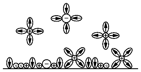
Figure 1: BDM model of charged double layer. Adapted from
[38,18]. The polar solvent molecules are shown
as ellipses, with the arrows pointing toward the positive end. The
specifically adsorbed (section 2.7) ions of
indeterminate charge are labeled as "q". Note that some of the ions are
solvated, which limit the closest approach distance.
If we apply a negative charge onto our electrode surface, then it will attract
positive ions from solution. This will have the effect of making the
charge of the electrode appear to be less negative to a test charge deep in
the bulk solution. This "charge screening" is exactly analogous to the
screening of point particles described by Debye, which is present in a broad
range of physical contexts. Charge screening is discussed again
in section 2.4.
Throughout this section, the potential far from the electrode (in
the "bulk solution") is set to zero. Relative to this potential, the
electrode is at an electric potential
.
The earliest model of the double layer was proposed by Helmholtz
[137,138]
in 1879.
He considered just the a layer of positively charged ions, tightly bound to
the negatively charged electrode surface. The centers of these ions were
postulated to lie on a
single "Helmholtz" plane at a distance
from the electrode surface.
The resulting potential is identical to that within a capacitor, and is a
linear interpolation between the electrode and bulk potentials, as shown in
2.2.
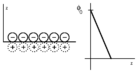
Figure 2: (a) Diagram of the Helmholtz model. The negative ions adsorbed
onto the surface are shown with solid lines. The positive "image"
charges are shown with dotted lines. (b) Potential
vs. distance
from the electrode.
An entirely opposite approach was undertaken by Gouy in 1910 [73] and
Chapman in 1913 [54]. They proposed that none of the ions were
tightly bound to the surface. Each ion is not constrained to lie in a tight
double layer, but is sensitive to the electric potential formed by the other
ions. In this way, the positions of the ions are not predetermined, but
are the
result of a statistical equilibrium with respect to this potential. This is
only a mean-field model; individual ions are expected to react only to the
overall field produced by all the other ions.
This mean-field model can be analyzed with some rigor.
First, the electric potential
depends on the charge density
as stated by Poisson's equation (in Gaussian units),
Then, (2.14) becomes
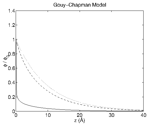
Figure 3:
Normalized potential profiles
vs.
for the
Gouy-Chapman model at
= 1000 mV (solid), 100 mV (dashed), 10 mV
(dotted). The
= 10 mV case is indistinguishable from the
limiting form (2.27) .
Note that larger values of
have steeper descents. I have used
the case of 0.1 M HClO
, just as in the experiments described later.
For this case, the Debye length is
= 9.6 Å. Adapted
from a similar figure in [19].
The Gouy-Chapman model is an improvement over the Helmholtz model, but it does
not take into account the finite size of ions. There must be a plane of
closest approach, just as predicted by Helmholtz. The minimum distance of
this plane from the electrode surface is the ionic radii. If the ions are
solvated, then they will not even be able to approach that closely. Stern
realized this in 1924 [125] and proposed a model to incorporate
this. Essentially, it is a combination of the two previous models.
Call the distance of closest approach
.
(OHP stands for "Outer Helmholtz Plane". The "Inner" plane will be
defined shortly.)
The Helmholtz description applies for
,
and the Gouy-Chapman description applies for
.
At this boundary, we require continuity in the potential
and its derivative.
In the
region, we have the Helmholtz linear potential drop
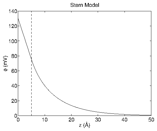
Figure 4: Potential profile
vs.
for the Stern model
at
= 130 mV. The transition point is set at
=
5 Å (dashed line), which then corresponds to a transition voltage of
= 75 mV. I have used the case of 0.1 M HClO
, as
in the experiments described later. Adapted from a similar figure in
[20].
We will discuss the following models only qualitatively. As we add more
components to the model, additional variables are added that are difficult
to measure. But it is important to keep the additional components in mind, if
only to appreciate the difficulty of predicting exact quantitative behavior.
The Grahame model [74] (1947) includes the possibility of ions
specifically adsorbed (section 2.7) on the electrode
surface. This specific adsorption is chemical in nature, and cannot be
explained simply by electrostatic arguments. These ions can have either
positive, negative, or no charge. We expect, however, that their ionization
state and degree of attraction to the electrode will be influenced by the
electrode's potential. The closest approach of these adsorbates defines the
"Inner Helmholtz Plane".
The Bockris-Devanathan-Müller model includes (polar) solvent molecules that
bring us to our complete picture shown earlier 2.1.
In retrospect, all of this model-building may seem somewhat ad hoc. A
contrasting approach has been put forth recently by
Borukhov et al. [36]. The
authors start with the
Poisson-Boltzmann equation but include the contributions to the free energy
from the finite size of the ions. This remediates some of the defects of the
Gouy-Chapman model and is in agreement with experiments they cite where large
multivalent ions are adsorbed onto a charged Langmuir monolayer.
4 Charged Ions in Solution
Having discussed the electrode surface and its ionic neighborhood, we turn to the charged ions in bulk solution. First, the various modes of transport of charged ions to the electrode surface are discussed and compared. These play an important role in the kinetics of deposition at that interface. Second, the importance of a supporting electrolyte in electrochemical experiments is described.4.1 Transport of Ions
In any deposition/growth system, the transport of particles to the surface is an important consideration. Often, the evolution of the surface morphology is determined by the relative rates of transport to the surface and reactions at the surface. Two familiar limiting cases are diffusion-limited aggregation (DLA) [153,154] and kinetic-limited growth (such as the KPZ model [86]). All electrochemical reactions take place only at the electrode surface, so transport of ions to that interface is of paramount importance. We expect the current of species to be proportional to its respective electrochemical potential gradient,Fick's first law can be derived by considering the Brownian motion of particles. A simple treatment can be found in [25], which considers a random walk of fixed step size. More sophisticated treatments make use of the Langevin equation [97]. Fick's second law of diffusion (2.36) follows from the first (2.35) by the continuity equation (2.33). The diffusion constant can be solved for by using a Fourier transform (appendix B)
4.2 Supporting Electrolyte and Charge Screening
In addition to the species of interest, most electrochemical experiments incorporate a supporting electrolyte. This is either the solution or is dissolved in the solution at a high concentration with respect to the species of interest. For instance, in our experiments the primary solution was H O, and the supporting electrolyte was 0.1M HClO . A brief and practical discussion of supporting electrolytes can be found in Brett and Brett [40]. There are several advantages to using a supporting electrolyte. First, the double-layer does not extend far into the solution; the majority of the potential drop is very close to the electrode (section 2.3). Second, ions are well-screened. As described by Debye-Hückel theory (see, for example, McQuarrie [98]), a charge in solution tends to attracts charges of opposite sign. The gives rise to an effective "ionic atmosphere" that diminishes the effective net charge felt by a test charge some distance away. Third, because there are far more charged ions in solution, the overall resistance of the solution is much diminished. Fourth, most of the current is carried by the electrolyte, not the dilute ions. This has implications on the dominant mode of transport. In any electrochemical system, it is important to determine what fraction of the measured current is derived from diffusion as opposed to electromigration. When both effects are present, the analysis becomes complicated. However, electrochemical experiments are generally carried out with a large concentration of a supporting electrolyte relative to the concentrations of active species. The supporting electrolyte does not take part in the reaction at the electrode, but does carry the majority of the current through the solution. The electrolyte serves to screen the ions, making the "ideal gas" approximation more realistic. Hence, the deposited ions arrive mostly via diffusion, and electromigration effects can be neglected [26].5 Bulk Deposition
In this section I will discuss the deposition of "bulk" amounts of material onto an electrode surface. In the next chapter I will turn to "underpotential" deposition, which occurs at voltages closer to the rest potential, and is sometimes the precursor to bulk deposition. As a prelude to understanding underpotential deposition, it is necessary to understand something about bulk deposition. First I will discuss the Nernst equation, which determines the onset of bulk deposition. Then I will introduce the Cottrell equation, which is a simple realization of bulk deposition. Both of these are covered in the more analytical electrochemistry texts.5.1 Nernst Equation
In discussing chemical activities (section 2.2) and and electrochemical potentials (section 2.2), we have already developed the necessary machinery to write down the Nernst equation. The following treatment parallels Bard and Faulkner [27]. Using the relation between chemical potentials and chemical activities (2.2), the Gibbs free energy iswhere the formal potential incorporates the activity coefficients. The formal potentials for various reactions can be easily measured and are tabulated in the literature. Bulk deposition is just an example of these reversible reactions we have been discussing. Consider the deposition of copper ions from solution onto an inert electrode. This is written as
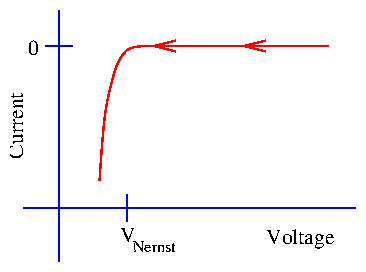
Figure 5: Cartoon of Bulk Deposition
5.2 Cottrell Equation
Consider a deposition experiment where the potential is abruptly shifted from above the Nernst potential (no deposition) to below the Nernst (bulk deposition). Before , the system is in equilibrium with a mean concentration of everywhere; . At , the voltage is altered such that deposition occurs. The electrode surface is assumed to be perfectly adsorbing so that it is a perfect sink for the adsorbing ions; . Each of these adsorbed ions transfers electrons to/from the electrode. Furthermore; the solution container is semi-infinite and hence inexhaustible. Far from the electrode, the bulk solution concentration will be maintained; . We must solve the linear diffusion equationThe standard method [28,41] is to Laplace transform (2.44) and the initial condition:
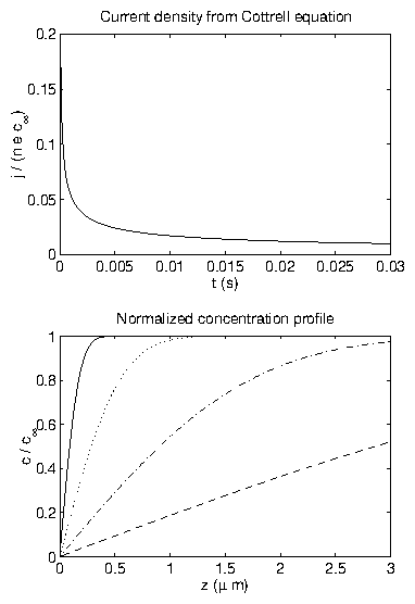
Figure 6: (a) Current density at the electrode surface from (2.53).
(b) Concentration profiles from (2.53), for
s (solid),
s (dotted),
s (dot-dashed), and
s (dashed).
6 Underpotential Deposition
Imagine that we start at the rest potential and slowly sweep the potential in a negative direction. In contrast to the cartoon of bulk deposition (figure 2.5), small peaks in the current response can be observed. This phenomenon is not ubiquitous. These peaks are only observed for particular species deposited onto particular electrodes. In addition, this phenomena is very surface-sensitive. For instance, the peak positions and heights when Cu is deposited onto Pt vary depending upon the particular Pt crystal face: (111), (100), or (110). This process is termed underpotential deposition, because the deposition takes place at potentials "under" the Nernst potential (closer to the rest potential). A potential applied beyond the Nernst potential is often termed the overpotential, as in (6.2).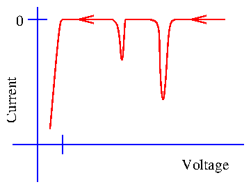
Figure 7: Indication of underpotential deposition during a voltage sweep.
Although underpotential deposition (UPD) is a complex process, we can
qualitatively justify this behavior. Presuming that a Cu ion has a greater
affinity to bond to a Pt atom than it does to another Cu atom, then we can
imagine that the underpotential deposition situation shown in the top panel
of figure 2.8 would be favored at some potentials for which
bulk deposition, shown in the bottom panel, would not. In the top panel, each
deposited Cu is directly in contact with the Pt surface. In the bottom panel,
the subsequent Cu layers are only in contact with the prior Cu layers.
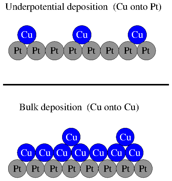
Figure 8: Difference between bulk deposition and underpotential deposition
In the next section, I present simple models of
"specific adsorption",
of which underpotential deposition is a particular example.
7 Specific Adsorption
In the discussion of the double layer (section 2.3) we considered the electrostatic interaction of charged ion species with the charged electrode. In our most sophisticated model, we assumed that no ion could approach closer than the radius of its solvation sphere. Ions that do lose their solvation spheres and penetrate within the outer Helmholtz plane are said to be specifically adsorbed. Their interaction is more than electrostatic, and is comparable to a chemical bond. Bard and Faulkner [29] make the analogy:Needless to say, these interactions will be very complex. Models of these processes need to combine the ionization of charges near surfaces, solvation, chemical bonding, charge-screening, and surface phenomena such as work functions.The difference between nonspecific and specific adsorption is analogous to the difference between the presence of an ion in the ions atmosphere of another oppositely charged ion in solution (e.g., as modeled by the Debye-Hückel theory) and the formation of a bond between the two solution species (as in a complexation reaction).
8 Adsorption Isotherms
Even in the absence of any adsorption, there would be some concentration (equal to the bulk concentration) of ions of species in a region near the electrode surface. The surface excess concentration [116,30] is defined to be the concentration of species in excess of the bulk concentration, normalized by the area of the electrode. The "coverage" is defined to be the surface excess normalized by its saturation value, , so that . The definition of this region "near" the electrode surface is somewhat arbitrary. In principle, it can include the diffuse double-layer. However, the in the diffuse double layer will have little effect if we have a supporting electrolyte. First, most of the the ions drawn into the diffuse double layer will be from the supporting electrolyte, not the species . Second, the width of the diffuse double-layer narrows exponentially as the concentration of ions increases. In the limit that the adsorbates on the surface to do not interact, we can write down a simple model for the adsorption onto a surface. This is very similar to standard the simplest lattice-gas models of adsorption discussed in introductory statistical mechanics courses. I also assume that there is no interaction between the species and the solution itself, and that there is no species-species interaction in the solution. If concentrations are not too high, then the supporting electrolyte screens these charges. The rate of adsorption is proportional to the concentration of ions in solution , the number of sites available for adsorption , and a Boltzmann factor involving the Gibbs free energy of the activated complex (see figure 2.9) and the Gibbs free energy of the ion in solution . Isotherms, by definition, are equilibrium measurements. Hence we usually assume that the system has come to equilibrium such that the concentration near the electrode is equal to that in the bulk solution, . We are also implicitly neglecting the diffuse double layer (which is described by the Poisson-Boltzmann distribution).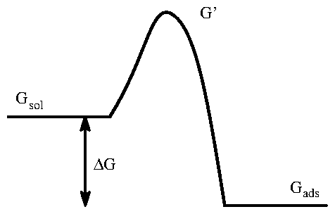
Figure 9: Diagram of energy levels for adsorption process.
In this case, adsorption is energetically favored by an amount
, but the system must first overcome an energy barrier
.
Similarly, the rate of desorption is proportional to the concentration on
the surface
and another Boltzmann factor involving
and the
Gibbs free energy of the adsorbed ion
.
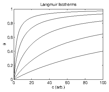
Figure 10: Langmuir isotherms for various values of
.
To make a slightly more realistic model, we assume that there is some
interaction between the adsorbates. Using a mean-field approach,
let
. If the adsorbates attract one
another, then
. If they repel, then
. In the case
that
, we recover the Langmuir result. Typically this isotherm is
written as
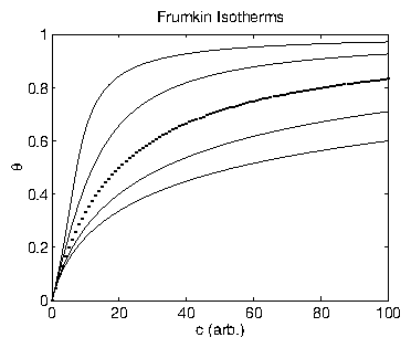
Figure 11: Frumkin isotherms for various values of
.
The dotted line corresponds to
, which is identical to the Langmuir
isotherm.
The choice of which isotherm to use depends upon experimental conditions. The
Langmuir isotherm is an accurate description for small coverages (
),
or equivalently, small concentrations. In this regime the adsorbates are
sufficiently sparse that they do not interact. Because of the approximation
used to derive it, the Temkin isotherm is only used for
and
not approaching zero. The Langmuir and Frumkin isotherms are
virtually indistinguishable as
, and both are linear in
that regime. These two points become apparent upon
expanding (2.57) in this limit and keeping terms to
second order,
Chapter 3
Introduction to X-ray Scattering
1 Introduction
This chapter provides an introduction to x-ray scattering, suitable for a first-year graduate student studying physics, chemistry, or a related field. It covers a broader range of material than is necessary simply to interpret the results in chapters 5 and 6. The reader may safely decide to skip ahead and return back to the specific sections that are referenced in those chapters.2 Generation of X Rays
Early x-ray experiments were performed with x-ray tubes, and today most still are. Presently there are at least two other available sources, both superior to tubes. Rotating anode sources, while expensive, can easily fit within a room. Synchrotron sources are extremely large multi-user facilities, of which only a handful exist in the world. The benefits include an enormous gain in flux and angular collimation. Both of these sources were used for this dissertation, and I will discuss them in turn.3 Conventional X-ray Sources
"Conventional" x-ray sources [57] work on the same principle as Röntgen's original apparatus; electrons are accelerated into an block of material (the anode), generating x-rays. While the x-ray tube of Röntgen used electrons ionized from gas, today the electrons are produced by a high-current filament. These electrons are then accelerated by an electric field into the anode. When struck by the electrons, the anode produces a broad, continuous spectrum of x-rays, due to the electron deceleration within the anode. This is typically called bremsstrahlung from the German "braking radiation". The more useful spectral components are the "characteristic" radiation lines, which arise from electronic transitions within the anodic atoms. If an electron kicks out an electron from an atom, the atom will be in an excited, ionized state. Subsequently, one of the remaining atomic electrons will fall into the unoccupied state, releasing an x-ray photon and conserving energy. Due to the quantized energy levels, the resultant x-ray spectrum is also discrete, and characteristic of the atomic element. The wavelengths are labeled according to the energy transition. For instance, the lines correspond to transitions from ( ) to ( ), the from ( ) to , and from to . The principal quantum number here is denoted by . These characteristic lines can be exceedingly narrow ( 0.001 Å), so it is possible to have nearly monochromatic radiation for an x-ray experiment. Sometimes it is even possible to resolve the lines even further. The , for instance, can split into the and . These correspond to transitions from states with slightly different energies (the fine structure). The intensity (per ) in the characteristic lines is higher than the bremsstrahlung by a few orders of magnitude. Nevertheless, the flux per solid angle is low because the radiation is spread isotropically into all directions. The overall intensity can be boosted by using the highest electron beam current possible. In practice, this requires both water-cooling the anode and rotating it to prevent a single focus spot from overheating. These rotating anodes provide the highest flux presently available in a "bench top" laboratory setting. For the work presented in this dissertation, a Rigaku (Model RU200) rotating anode was used primarily for orientation of samples, training, and as a testing bed for the experiments. This instrument has a tungsten filament that can support up to 200 mA current. The electrons are accelerated over potentials as large as 60 kV into a rotating, water-cooled copper anode.4 Synchrotron X-ray Sources
A synchrotron x-ray source begins with an ultra-high vacuum (10 Torr) storage ring. Within the ring are electrons circulating at near-light speeds. Whenever a charge is accelerated (for instance, if constrained to a circular path) it emits radiation. In doing so, it loses energy. To keep the electrons moving in stable orbits, energy in the radio frequency range is added at intervals synchronized with the electron "bunches". While electromagnetic radiation is produced for any acceleration, it is advantageous to place additional accelerating devices at specific locations. In our experiments, these were simple "bending magnets" that sharply steer the electron beam. More sophisticated devices, such as "wigglers" and "undulators" cause the electron beam to be accelerated up and down several times within a narrow spatial region. This leads to a corresponding increase in the intensity of the overall x-ray beam delivered. A brief, if dated (1979), review of synchrotron radiation can be found in [56]. An even shorter overview is presented in [87]. A thorough and very recent (not yet in print) account of synchrotron radiation and related devices is [77]. The remainder of this section will use a few results derived in [130]. The most striking feature of synchrotron sources is the high degree of collimation (unlike conventional sources, which radiate into all solid angle). The "opening angle" for the radiation is peaked sharply forward and determined by the speed of the electrons. The full-width at half-maximum is [130]5 Single-Electron Scattering
Although x-ray scattering is inherently a quantum phenomenon, many important features can be correctly derived from a classical treatment [141]. A quantum mechanical treatment can be found in [46,112]. We will also take the nonrelativistic limit and use Gaussian units. Following the general treatment in [82] assume a "free" charge of magnitude and mass . This is subject to an incident electromagnetic plane wave of frequency , wavevector , electric field amplitude , and polarizationAs usual for electromagnetic radiation, , , and are mutually orthogonal. By the Lorentz force law and Newton's second law, a free point charge will then accelerate as
so the radiation will be an electromagnetic spherical wave, of the same frequency. The "ret" refers to the fact that the quantities within the square brackets must be calculated at "retarded" time . Writing the electric field more definitely,
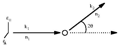
Figure 1: Diagram for classical x-ray scattering
Take
and
to define the "scattering plane",
and define
the angle
to lie between them:
6 Scattering from Multiple Objects
In this section, I will discuss scattering from multiple objects. By considering the phase difference between scattered waves from spatially separated objects, I introduce the structure factor. Then I discuss the connection between the structure factor and the correlation function.6.1 Fourier Transforms
I assume the reader is familiar with the use of Fourier transforms. This section merely defines the Fourier transform as I will use it, as there is some variety in the normalization and sign conventions in the literature. Throughout this dissertation, the Fourier transform of a function in dimensions is defined to be6.2 Structure Factors
Take the cross section derived in (3.15) and let the charge equal the charge of an electron, . Defining the classical electron radius, = 2.818 10 Å, we have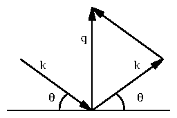
Figure 2: Diagram illustrating that
.
For elastic scattering, the incoming wavevector
and
outgoing wavevector
both have length
. The momentum
transfer
. From
[9].
6.3 Correlation Functions
I will define the two-point correlation function (also known as the pair correlation function) asThe significance of this result is that if we could measure for all , we could completely determine the correlation function . In practice, unfortunately, we can only measure for a limited range of angles and lengths of . This limits our knowledge of . Because it is a convenient abbreviation that I will use in section 3.10, let me mention one more relation.
7 Scattering from Atoms
Previously (section 3.5), we discussed the scattering from a free electron. In this section, we consider the x-ray scattering from an atom, based upon references [2,58,59,60,142,143]. As shown in (3.15), a particle's cross section depends on its mass as . Since the proton/electron mass ratio is over 1800, the x-ray scattering from the nucleus is miniscule, and is usually neglected. Ultimately, we would like to have a function, the atomic form factor, which accounts for all the subatomic structure, and tells us how the scattered amplitude is modified (compared with the case of a single free electron). Because this is a common desire, these functions are tabulated in standard references [152,1,2]. If we consider just the electron probability density cloud surrounding the nucleus and approximate each of the electrons as being free, then we arrive at the standard form factor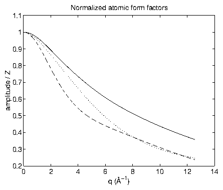
Figure 3: Standard atomic form factors
, normalized by atomic number
, for Pt (solid), Cu (dotted), and Cl (dashed). Note that
. From [151].
However, the free-electron assumption is only an approximation, and fails most
noticeably near "adsorption edges". When the x-ray energy is tuned close to
an absorption edge, it can eject a core-level electron from the atom. (This is
related to the electron-induced ionization discussed in
section 3.3).
Deviations of the measured form factor
from
are known as as
"anomalous dispersion". Typically, this modification to the amplitude is
separated into a real term
and an imaginary term
. The
latter term allows for a change of phase in the scattered beam and is
manifested as absorption. Physically, the anomalous dispersion arises from
the resonance of the incident x-ray with differences between atomic energy
levels.
Summarizing the various terms that comprise the atomic form factor
:
7.1 Absorption
Absorption of x-rays is caused by an incident x-ray striking an atom and causing a core level electron to be ejected [61]. This is simply the photoelectric effect, which is usually presented in the context of ultraviolet photons incident upon the outer shells. Historically, this was one of the most dramatic experiments leading to the quantum paradigm. After the photoelectron is ejected, the atom is in an excited state. Just as described in section 3.3, an electron will fall into the vacated state and emit a characteristic x-ray; this process is called "fluorescence". Because the electron falls from an atomic level and not from the vacuum, the fluorescence energy is always less than the energy of the absorbed x-ray. Empirically, the absorption of x-rays by matter is observed to be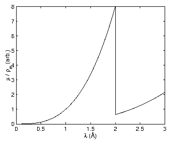
Figure 4: An illustration of a mass absorption coefficient vs. wavelength.
This is intended only for illustration, so it corresponds to no element.
The sharp drop in intensity is known as the absorption edge.
8 Crystals
A Bravais lattice is the set of points that can be reached from a single point by applying translation vectors. These translation vectors are called "basis vectors" and are equal to the number of dimensions of the space of the lattice. For real crystals described by Bravais lattices, there are three basis vectors. Calling these basis vectors , , , the Bravais lattice consists of the set of vectors ,9 Diffraction from Crystals
9.1 Infinite Crystal
Consider an infinite array of point chargesFor nonzero , we thus require the Laue conditions
where the indices , , span all of the integers. These conditions define a lattice of points in reciprocal space. These points are just the reciprocal lattice described by (3.52), as we can show with a simple example. The vector is just
This is equivalent to , the definition of the reciprocal lattice (3.52). We might choose another basis for , instead of (3.64), but will remain the same. So, the diffraction pattern from a Bravais lattice is its dual reciprocal-space Bravais lattice. Take as the projection of a given along . This is the distance between two planes of the lattice. From and the definition of (3.30), we recover Bragg's law:
9.2 Lattices with a Basis
In this dissertation, we will be most concerned with the structure of platinum. This is a face-centered cubic crystal, which can be visualized as a cubic crystal with an extra atom at the center of each of the cubic faces. Some crystal structures are not Bravais lattices , for example, silicon and diamond. They can, however, be described as a face-centered cubic crystal with another face-centered cubic crystal superimposed upon it. The second lattice has a relative displacement of along the cubic body diagonal. The "diamond structure" is described by vectors that run over the Bravais lattice, but also include the basis vector for this displacement. Although the face-centered cubic structure is a Bravais lattice, it is convenient to describe it as a simple cubic lattice with a basis. The basis vectors in this case describe the atoms on the faces. For a simple cubic crystal with basis vectors , , and , the displacement basis vectors that generate the face-centered cubic crystal areFor a crystalline sample, we can divide the space into unit cells that are repeated over all Bravais lattice vectors. Then we can consider the scattering from one unit cell and replicate it over the Bravais lattice. For the face-centered cubic crystal, the scattering amplitude due to one cube is
So the diffraction pattern will be identical that of a simple cubic lattice, except that intensity at values which are all odd or all even will be enhanced, and the intensity at other values will be extinguished.
10 Thermal Effects and Inelastic Scattering
This section is based upon [11,63,145,146,47]. Consider an ideal crystal as in (3.53),and allow the atoms to oscillate about their respective mean positions such that their instantaneous positions are . Then,
Thus, x-ray diffraction measures the static structure factor automatically. Although sometimes called elastic scattering (because there is no energy dependence), this is a misnomer. In fact, we are integrating over all energy transfers , not selecting out the elastic ( ) term.
11 X-ray Scattering from Surfaces
X-ray scattering from surfaces is usually presented in either of two ways. In section 3.11.1, I present the method of truncating an infinite crystal, popularized by Robinson [111]. The following section (3.11.2) describes the more traditional approach from classical electrodynamics. The final section (3.11.3) establishes the connection between these two approaches.11.1 Truncating the Infinite Crystal
This section builds upon the treatment of the infinite crystal in section 3.9, and extends it to semi-infinite and finite crystals.11.1.1 Semi-Infinite Crystal
In analogy with (3.54), consider an ideal semi-infinite crystal. One face of the crystal is presumed to be truncated at while the opposite "end" stretches to infinity. As before, we begin with the one-dimensional case, which illustrates the relevant behavior.11.1.2 Finite Crystal
Now, we truncate the crystal at both ends, so that it is a one-dimensional crystal containing scatterers. Using the relation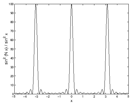
Figure 5: Graph of
vs.
, for
.
The structure factor here is just like the diffraction intensity from
a diffraction grating with
slits (shown in figure 3.5).
Near the Bragg diffraction peaks
(
), the limit
.
Because the crystal is finite, the structure factor maxima are now
, not
infinite. The minimum value is zero, which is also in contrast with the
semi-infinite crystal, but identical to the infinite crystal.
The extension to three dimensions is straightforward [111].
Consider a three-dimensional crystal with
,
,
scatterers in
the
,
,
directions.
The scattering amplitude is then
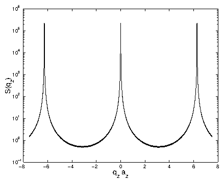
Figure 6: A logarithmic plot of
vs.
as given in
(3.92) for
. This is the same
function shown in figure 3.5, but with a larger
. Also,
a finite
resolution function has been convolved through the data. This eliminates
the numerous minima seen in figure 3.5, and is
reasonable from an experimental standpoint. The minimum value is near
, because
. Without the convolution,
the minimum value is zero.
11.2 Reflectivity from Smooth Surfaces
An alternative treatment is to consider x-ray scattering from a surface as an example of the more general problem of reflection and refraction at a boundary between two dielectric media. Since x-rays are just electromagnetic radiation, this should be perfectly valid. For the moment, however, we neglect the atomistic nature of the sample and assume it to be a smooth, continuous structure. The atomic periodicity can be added in later (section 3.11.3).11.2.1 Fresnel Equations
Consider a smooth interface between air ( ) and a block of amorphous material ( for x-rays). This ties into the classical electrodynamic treatment described by Jackson [84], with , , and . Jackson uses , the angle between the incident beam and the surface normal. For consistency with the rest of the dissertation, I write results in terms of its complementary angle between the incident beam and the surface.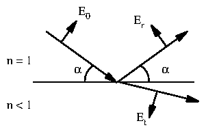
Figure 7: Diagram for the Fresnel equations.
and the parallel components are
The Fresnel reflection and transmission coefficients are plotted in figure 3.8. If , as we will show is true for x-rays incident on most materials, then there exists a critical angle such that . For , , so the square roots become imaginary and the magnitude of is unity for both polarizations. This is termed total external reflection.
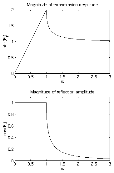
Figure 8: Fresnel reflection and transmission coefficients.
In this example,
.
The transmission is sharply peaked at the critical angle, then
quickly falls to unity.
11.2.2 Index of Refraction
While a long derivation of the index of refraction can be found in Warren [147], a simpler and more illuminating treatment can be found in Jackson [85]. I will not repeat the entire model here, but just connect the results to our discussion. For large enough photon energies ( ), the dielectric constant approaches the "plasma limit" and11.2.3 Critical Angle Calculations for Platinum
As an example, the critical angle for platinum is calculated in this section. The atomic weight of platinum, , is 195.078 g/mol, its atomic number = 78, and the mass density = 21.090 g/cm . Hence, the density of electrons in platinum is11.3 Scattering and Reflectivity
There are some apparent disparities between the results of the CTR theory (section 3.11.1) and the classical Fresnel reflectivity (section 3.11.2). The former predicts Bragg peaks connected by crystal truncation rods. Given no adsorption and a truncated infinite crystal, these Bragg peaks are predicted to have infinite intensity. The Fresnel formulae have no Bragg peaks or truncation rods, and the intensity maximum saturates at unity below the critical angle. The Fresnel treatment cannot predict Bragg peaks, because the scattering media is assumed to be a solid block of constant density. The CTR treatment assumes a perfect crystalline lattice. If we extend the CTR treatment to consider continuous, homogeneous media, then integrals will take the place of summations. The scattering amplitude isSince , and the Fourier transform of unity is a delta function, then Fourier transform of the step function is finally
In fact, even without knowing (3.109), one can show just from (3.110) that if , then . The result can be obtained in two other ways. Taking the continuum limit of the semi-infinite structure factor (3.85) yields this directly. The second method is to follow [124] and consider the structure factor (3.31) again:
Chapter 4
Experimental Procedures and Apparatus
1 Introduction
In this chapter, the specific procedures and apparatus used in these experiments are documented. First, the sample preparation protocol is described. The next section details the electrochemical apparatus and procedures. The following section describes the x-ray scattering apparatus, and the timing apparatus is discussed thereafter. Finally, suggestions for future improvements are made.2 Sample Preparation
2.1 Procurement
Samples (nominally Pt(111)) were obtained from the Materials Science Center growth facility in Bard Hall. These samples were oriented through Laue back reflection, and then cut to the desired orientation by electrical discharge. Then, they were polished with SiC paper and Al O powder down to a grit size of 0.25 m until a mirror-like surface was obtained. In principle, this procedure should produce crystals with well-oriented faces. To allow large terraces to form on metal crystals, it is desirable to reduce the miscut angle between the crystallographic axis (e.g., (111)) and the surface normal. However, miscut angles as large as 2 were measured in our lab by a combination of laser reflection and high-resolution Bragg diffraction. These can be traced to the Materials Science Center crystal mounting apparatus, which was insufficiently rigid to ensure a miscut smaller than a few degrees.2.2 Miscut Calculation
In this section, the angle is the Bragg diffraction angle, while is a rotation angle about the surface normal. On a miscut crystal, the Bragg diffraction peak will not be coincident with the surface normal. The angle between them is defined to be . The surface normal was aligned with the axis as follows. By reflecting a laser beam from the mirror-like face of the crystal, a tight spot was cast onto a far wall or ceiling. Rotating the crystal about caused the laser beam to trace out a cone, causing the spot to trace out a corresponding ellipse on the wall. By adjusting the tilt stages on the sample goniometer, the ellipse could be narrowed until the spot did not move with . Then, the surface normal was well-aligned with the axis. Moving the angle to some fiduciary value, such as 0 , the Bragg diffraction angle was recorded. Then, was set to 180 and a different was found. These two angles differ because the diffraction peak traces out a cone, similarly to the laser beam. The projection of the miscut along this one axis is (see figure 4.1)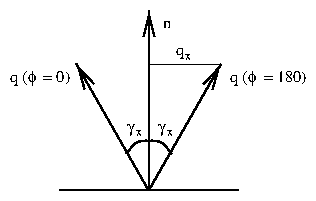
2.3 Sample Preparation
After the miscut of each platinum crystal was measured, it was mounted onto the orienting/polishing apparatus shown in figure 4.2. The apparatus consists of a cylindrical barrel (E), with three dowels mounted on it (C). (Only two dowels are shown in the figure.) These form one half of the "kinematic mount"; the other half is a thick disk (B), into which the dowels press. Opposite the first dowel is a circular depression (G), opposite the second is a groove (H), and opposite the third is just the flat surface of the disk. One of the dowels is fixed; the other two can be raised and lowered my means of small adjustment screws running through the barrel. These permit the disk to be oriented by a few degrees in any direction with respect to the barrel axis. A long screw (D) attached to a spring and knurled knob (F) runs through the barrel axis and passes through the clearance hole (I). When tightened, the orientation is securely fixed. Finally, a mushroom-shaped tip (A) fastens to the kinematic disk (B) with three screws. The sample fits on to the end of this tip.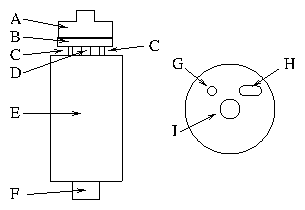
Figure 2: Diagram of orienting/polishing apparatus. (a) Side view. (b)
Bottom view of the stage (B), showing the kinematic mount. Labels are
described in the text.
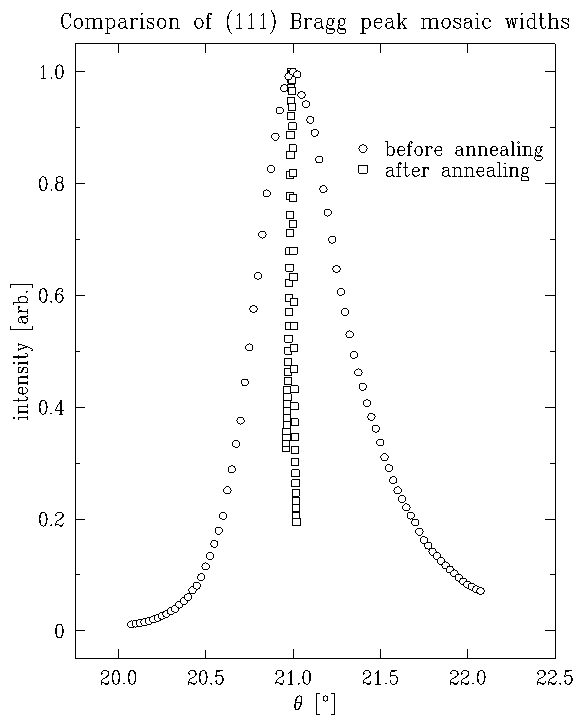
Figure 3: Mosaic scans, before and after annealing, normalized to unit peak
height.
After several iterations of this orienting-polishing-annealing
procedure, the bulk mosaic of the platinum
crystal was
(full-width at half-maximum) and the
surface normal was oriented to within
of the (111) direction.
Empirically, we have found that both the mosaic and the miscut must be small
in order to observe the incommensurate overlayer. Furthermore, a high quality
substrate enhances the quality of voltammetric profiles.
The development of this procedure was crucial to the success of this
experiment. It has also propagated to other
groups (Cooper, Ho) in Clark Hall, and has enabled them to improve surface
quality and signal-to-noise ratios in their own data.
3 Electrochemical Apparatus and Procedures
3.1 Solutions
Most of the solutions were prepared by Lisa Buller, and the following paragraph is paraphrased from her dissertation [52]. All solutions were prepared using water purified by a Hydro purification train and a Millipore Milli-Q system. The ionic salts were used as received and always the purest available. Perchloric acid solutions were prepared by dissolving either CuO (99.999%, Aldrich) or CuCl (99.999%, Aldrich) in Ultrex perchloric acid. The addition of chloride anions was achieved through the addition of CuCl or NaCl (99.999%, Aldrich). All solutions were bubbled for at least 15 minutes with pre-purified nitrogen, which was further purified by passage through oxygen-absorbing (MG Industries Oxisorb) and hydrocarbon (Fisher Scientific Activated Carbon 6-14 Mesh) traps to remove all traces of oxygen.3.2 Three-electrode Electrochemical Cells
A typical well-designed electrochemical cell has three electrodes [118,43,44]. The guiding principle is to have all the interesting behavior occur at the working electrode. The other electrodes should be relatively inert and not complicate the analysis of the processes that occur at the working electrode. All potentials must be measured relative to some other reference value, which is provided by the reference electrode. The perfect reference electrode would be "ideally nonpolarizable". That is, its potential remains constant, regardless of the amount of current passing through it. Another purpose of the reference electrode is to ensure that an applied potential change does what we expect. Suppose we change the voltage of the potentiostat by . How do we know that this causes a at the working electrode and that part of the does not go into the reference electrode? If the reference electrode is ideally nonpolarizable, it maintains the same potential value, and the full is effected at the working electrode interface. The counter (or auxiliary) electrode assists in this process. If the reference electrode is passing a significant amount of current, then the assumption of ideal nonpolariziability is sorely tested. It is preferable to have an alternate, low-resistance, pathway through which most of the current flows. Counter electrodes are often composed of inert metals and have large surface areas to minimize their overall resistance. The various electrodes used in our experiments are shown in figure 4.4. The large (10 mm) electrodes used for the simultaneous in situ x-ray and electrochemical measurements are labeled by (a). The smaller (1-2 mm) "ball" electrodes, labeled by (b), were produced by members of the Abruña group. These were of excellent quality, and produced good electrochemical signals. However, they were too small and too difficult to orient to be of use in our x-ray measurements. A Ag/AgCl reference electrode is labeled by (c). These were constructed by Lisa Buller [52].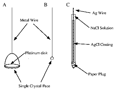
Figure 4: Electrodes used for the electrochemical measurements. (A) 10 mm
diameter electrode. (B) 1-2 mm diameter electrode. (C) Ag/AgCl
saturated-NaCl reference electrode.
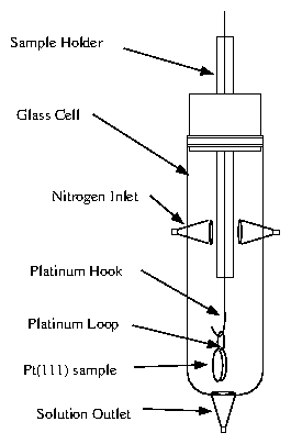
3.3 Hanging Meniscus Cell
For electrochemical experiments on single crystals, a hanging-meniscus cell is ideal. A wire is spot-welded to the sides of the crystal face, as in figure 4.4(a,b). The face of the crystal is then dipped into the solution compartment (see figure 4.5), and pulled upwards so that only a meniscus connects the sample with the bulk of the solution. The reference and counter electrodes are placed in another compartment, connected by a frit (partially fused glass). The advantage of this arrangement is that only the crystal face of interest in contact with the solution. Also, it is easy to use small (a few mm diameter) crystals, which are often better quality than large (10 mm diameter) crystals. The disadvantage is that the cell must remain in a fixed vertical configuration; this requirement is incompatible with most x-ray diffractometers. We used this cell only for voltammetric and current transient measurements.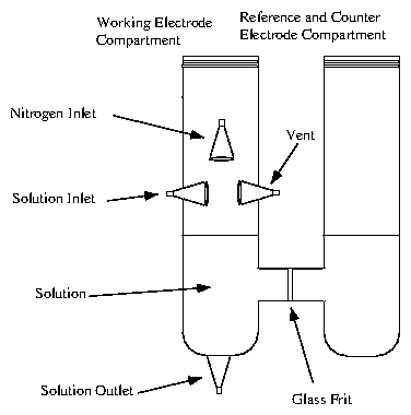
3.4 In Situ X-ray cell
To perform simultaneous electrochemical and x-ray measurements, we constructed a cell similar to the one developed by Toney and coworkers [113]. This is a reflection-geometry cell, as shown in figure 4.6. The entire sample is immersed in solution, unlike the hanging-meniscus cell. The solution is contained by 6 polypropylene film, held in place by an O-ring.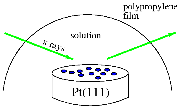
Figure 6: Cartoon of in situ electrochemical x-ray cell.
A detailed illustration of the cell is provided by
figure 4.7. The majority of the cell is Teflon
(Kel-F is an alternative material with greater strength). The sample is
placed in the center and held in place by two non-circular Kel-F screws that
squeeze the sample laterally. The sample and screws are raised with respect
to a trough, where most of the solution resides. The reference electrode is
inserted from the side. The counter electrode is a platinum wire that
circumnavigates the trough several times.
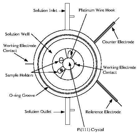
Figure 7: Detailed plans for the in situ electrochemical x-ray cell,
prepared by Lisa Buller [52].
3.4.1 Absorption
The x-ray reflection geometry places a limit on the in situ x-ray cell. The polypropylene film is extremely thin, and while contributing to the diffuse x-ray scattering background, does not We must incorporate the absorption of x-rays due to the layer of solution that is covering the sample. Consider an adsorbing layer of thickness and attenuation per unit length . From figure 4.8, the total path length of x-rays through the solution layer will be , where is the angle of incidence, and is the angle of reflection. For grazing incidence (small ), is limited by the horizontal dimensions of the sample. In the specular ( ) case, we have . From the relation (3.30) and the absorption relation for the intensity (3.48), then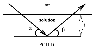
3.5 Potentiostat
A potentiostat is an instrument to keep the sample under potential (voltage) control and monitors the current. (A galvanostat, in contrast, keeps the sample under current control and monitors the voltage.) The simplest possible potentiostat circuit for a three-electrode configuration is shown in figure 4.9. The operational amplifier will supply sufficient current to keep the reference electrode at a potential with respect to ground (or the working electrode). Significant current will pass from the counter into the working electrode, but very little will pass through the reference electrode. This is in accordance with section 4.3.2.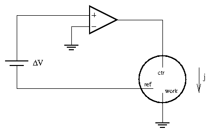
Figure 9: Simple potentiostat circuit for a three-electrode electrochemical
cell.
Adapted from [21].
3.6 Safety
In a dilute (0.1 M) form, perchloric acid poses a minor health hazard. Contact with skin is mildly irritating, and should be rinsed off as soon as possible. Contact with the eye is more serious. For this reason, splash goggles should be worn at all times. In case of a large spill, sodium bicarbonate should be available for neutralization. The platinum sample glows yellow-white during annealing. There is a significant ultraviolet spectral component, and the sample needs to be kept under continual supervision. To prevent permanent retinal damage, ultraviolet-resistant goggles must be worn during this process.3.7 Sample Treatment
Before a sample is inserted into the x-ray cell, a careful protocol must be observed. UPD is extremely sensitive to chemical contaminants, especially metallic and organic ones.- Spot-weld a clean platinum to the side of the sample, if not already present.
- Clean the top of the cell with solution; it should bead over everything. Then drain it away.
- Rinse the cooling cell with solution at least three times, draining with forced nitrogen.
- Have nitrogen flowing into the cooling cell.
- Flow solution into the cell, allowing a bubble to form on top of the cell.
- Put the hood (which should have nitrogen flowing through it) over the cell.
- Wear goggles to prevent retina burn.
- Anneal for 8 minutes the first time, 5 minutes each subsequent time.
- Cool in cooling cell for 4 minutes (under nitrogen overpressure).
- Flow solution into the cooling cell; fill to the level of the input port. Immerse the sample for at least one minute; a longer period is acceptable.
- The platinum surface will oxidize very quickly. The next step must be done very quickly!
- Remove the sample from the cooling cell and transfer it to the x-ray cell. To buy time, it is often helpful to squirt some solution or (deoxygenated) water on the face.
- Tighten Kel-F screw to fix sample in place.
- Cover with polypropylene film, which should be pre-rinsed. Cover with the O-ring and metal sleeve. Screw down the four jeweler screws evenly, for even pressure along the O-ring.
- The rest potential (no external potential applied) should be near 650 mV.
- With solution layer extended, run a cyclic voltammogram from 650 mV to 200 mV at 5 mV/s.
- With a syringe, pull out most of the solution and run an identical cyclic voltammogram.
4 X-ray Apparatus
X-ray scattering is a nearly ideal probe of the ordering kinetics of the two-dimensional overlayers found in UPD systems. Unlike electrons or neutrons, X-rays can penetrate through a thin solution layer, allowing the experiments to be performed in situ. X-rays provide structural information on atomic length scales without perturbing the system with mechanical probes or large fields, as scanning probe microscopes may. Finally, the extremely high flux from a modern synchrotron x-ray source, such as the National Synchrotron Light Source (NSLS), permits the weak diffraction signal from a single Cu-Cl bilayer to be studied at high resolution. In our experiments, the white beam produced by a bend magnet on the NSLS electron storage ring was focused in both transverse directions by a total external reflection mirror. A monochromator consisting of two Ge(111) crystals was configured to select 8.80 keV x-rays. The substrate was placed in a thin film geometry x-ray cell similar to those used by Toney and coworkers [113]. The cell was placed at the center of rotation of an Eulerian cradle and two pairs of XY-slits between the sample and the detector determined the resolution of the scattered x-rays. The resolution is discussed in detail in section 5.5. In the lab, x-rays were produced by a Rigaku (Model RU200) rotating Cu anode source. The Cu K was selected by means of either a single or triple-bounce Si(111) monochromator. Although the instrument can provide a 60 kV accelerating voltage and 200 mA filament current, the lowest power setting (20 kV, 10 mA) was usually sufficient for sample orientation. To detect x-rays we used an integrated NaI scintillation crystal, photomultiplier, and preamplifier (Bicron 1XMP 040B-X). The resulting electrical signal was sent through a combined amplifier and pulse-height analyzer (Canberra Model 1718) for broad energy discrimination. The TTL pulses were then sent to a simple adding memory module (Kinetic Systems 3610 Hex Counter) that also received timing pulses from another module (Kinetic Systems 3655 Timing Generator). In the lab, the signals were then acquired by a data acquisition card (DSP 6001). At the NSLS, data acquisition was handled by a CAMAC to SCSI interface module. In both places, the four-circle diffractometer (Huber) was under the control of a sophisticated software package ("spec", by Certified Scientific Software) running on an Intel 486-based computer.5 Time-Resolved Measurements
Time-resolved x-ray measurements can be accomplished in several ways. For instance, Bergmann et al. [32] used the timing of the electron bunches around the synchrotron ring for Mössbauer experiments. This is ideal for extremely short time ranges. Very recently, Knight et al. [88] have demonstrated a prototype device etched onto a silicon wafer to study protein folding. This works by mixing two jets together (for instance, folded protein and a denaturing agent) and squirting the product through a long channel. Because the flow is lamellar, the mixing occurs by diffusion. Because the fluid volumes are extremely low (nanoliters), the diffusive length scale is extremely short, and the mixing time is on the order of microseconds. By moving the device along the x-ray beam, different times after the mixing event are examined. In this way, position and time are coupled. In contrast, our method relies upon timing electronics to separate the x-ray signal into various time bins. This "stroboscopic" method was first used by our group to study charge-density wave kinetics [127]. Although the PAR 283 claims to have a trigger, it does not operate in the standard sense of the term. Normally, when an instrument (an oscilloscope, for example) is waiting for an electronic trigger, operation ceases until the trigger is detected. Then, the other operations are begun or resumed. Instead, the PAR 283 performs a variety of operations, periodically polling the input to see if the trigger signal has arrived. Only then is the specified series of actions initiated. This can lead to an unpredictable delay between the trigger input and the initiation of commands by the PAR 283. For this reason, it was decided to have the PAR 283 be the master controller and send trigger signals to the other instruments. The control diagram is shown in figure 4.11. The potentiostat applies a voltage to the sample and continuously reads current from it. At the beginning of a voltage cycle, it sends a trigger pulse to the waveform generator (Keithley 3940 multifunction synthesizer). This sends a series of pulses to the multichannel scaling averager (DSP 2190), which consisted of a multichannel scaling module (DSP 2090) and a signal averaging memory (DSP 4101). These bin pulses both initiated the averaging memory and incremented the current memory location (time bin). These timing modules also received x-ray intensity data, which was added to the time bin. At the end of a series of voltage cycles, the memory was dumped to the computer for display and analysis. The chronoamperometric traces (current vs. time) were digitized into 5000 time bins, and collected by the potentiostat. At the end of the voltage cycle, these were also sent to the computer.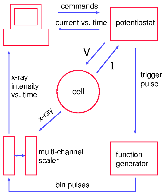
Figure 11: Instrumentation for timing experiments.
6 Future Improvements
6.1 New Cell Design
With the advent of high-energy synchrotron sources, x-ray cell geometries with a thick solution layer have become feasible. Brossard et al. [49] describe a cell very similar to ours, but without the thin solution layer constraints. The cyclic voltammetry measurements they present are not high quality; presumably, this is a function of sample preparation, and not the cell itself.6.2 Improved Sample Quality
As discussed in section 4.2.1, these crystals were not ideal. The simplest course would be to procure samples from a reliable external source. If annealing is still necessary, a new method should be found. Heating with a torch sometimes produced cloudy spots in the center of the sample, where the flame was hottest. A more even annealing could be done in ultra-high vacuum and by attaching it to a heating stage.6.3 Area (or Linear) Detectors
In our experiment, the highest resolution (section 5.5) was obtained by rotating the sample about the surface normal. In this case, an area or linear detector would not be helpful. However, there may be cases in which the resolution is sufficient to simply have an area detector mounted on the end of the detector arm. A CCD (charge-coupled device) could be run in a mode such that each line is shifted down. In this case, all of the time-resolved data could be recorded on the device, which would speed up the data acquisition time by the number of -points.6.4 Improved Electronics
In retrospect, the PAR 283 potentiostat was difficult to program, and not as flexible as anticipated. A superior solution would be to purchase the best possible analog potentiostat (BAS is an good choice) that accepts an external line voltage. Then buy a good programmable digital-to-analog card that can be programmed easily and has sufficient time resolution. It may also be advantageous to replace CAMAC modules with cards within the computers. At the time of these experiments, we needed to maintain compatibility with equipment at CHESS and NSLS X20A. Now, the DSP timing modules could be replaced with a multichannel scalar card (Oxford MCS, for instance). The counter/timer modules could be replaced with an integrated counter/timer card (Keithley CTM-010). These particular upgrades are already underway for the new spectrometer being set up in the Brock group laboratory.
Chapter 5
Cyclic Voltammetry and Static X-ray Measurements
1 Introduction
This chapter begins the presentation of our data on the underpotential deposition (UPD) of Cu onto Pt(111) in the presence of Cl. The first section presents our cyclic voltammetry on this UPD system. Subsequent sections discuss the hexagonal coordinate system and the structure of the incommensurate UPD overlayer. Finally, our static x-ray measurements of this overlayer are presented.2 Cyclic Voltammetry
Cyclic voltammetry, as the name suggests, is a measurement of the current while the voltage is being swept (usually linearly with time). The cyclic adjective refers to the fact that the voltage is swept in both directions. As a function of time, the applied voltage traces out a triangular wave (figure 5.1a). Cyclic voltammetry is a commonly used technique in electrochemistry, with many different applications. The next section illustrates a simple example: the cyclic voltammogram from an adsorption / reduction reaction, where the adsorption follows a Langmuir isotherm. In our experiments, this technique provided information on the equilibrium phase diagram.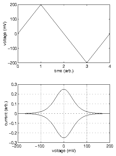
2.1 Cyclic Voltammetry for an Ideal System
This section follows the theory presented in section 2.8. It may be helpful to review that section before continuing. As suggested by Bard and Faulkner [31], consider the reduction of species O at the electrode to form species R.2.2 Cyclic Voltammetry for Cu/Cl/Pt(111) UPD
The voltammetric profile is shown in figure 5.2. These data were collected in our x-ray scattering cell at mV/s with M HClO as a supporting electrolyte, mM Cu and mM Cl . The current response exhibits two sharp and well-defined voltammetric deposition peaks centered at about and V (vs. a Ag/AgCl reference electrode). Upon reversing the potential sweep, the current response then exhibits two sharp stripping peaks corresponding to the reverse reactions.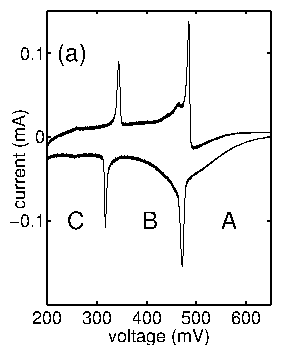
Figure 2: A cyclic voltammogram taken in the x-ray scattering cell at a sweep
rate of
5 mV/s with
mM
Cu
and
mM Cl
, and
M HClO
as a supporting
electrolyte.
A schematic of the deposition process is depicted in
figure 5.3.
The labels A, B, C in this figure also correspond to the potential regions in
figure 5.2.
At the rest potential (region A),
chloride anions are adsorbed on the platinum surface
in a non-ordered fashion [158,108].
As the potential is swept negatively,
copper is electrodeposited onto the platinum surface at a
well-defined potential
[90,149,94].
The electrodeposited copper and chloride ions together form an ordered
Cu-Cl bilayer structure incommensurate
[131]
with the platinum surface
(region B).
If the potential is then moved further in the negative direction,
there is further
copper deposition,
creating a full, commensurate copper monolayer
(region C) [94,90,156,157,95,72].
The copper
monolayer is, in turn, believed to be covered by a disordered layer of
chloride anions.
On the reverse (positive-going) sweep the reverse processes take place;
that is, some copper desorbs,
forming the CuCl lattice structure (region B) and at
more positive potentials the copper is completely stripped from the surface,
leaving the disordered chloride anions adsorbed on the surface
and returning the system to region A.
The sharp voltammetric features seen in Figure 5.2
are the electrochemical signature of a
clean and well-ordered surface.
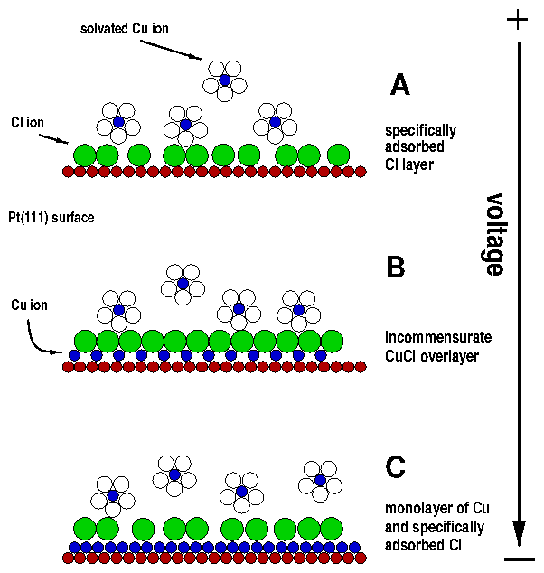
Figure 3: Cartoon of phases in the UPD of Cu on Pt(111) in the presence of
Cl.
In our experiments, we used cyclic voltammetry for three purposes. Most
importantly, it served as a qualitative "fingerprint" of the UPD process
itself. The cyclic voltammograms are extremely sensitive to contamination of
the solution, poor quality of the single-crystal electrode surface, and
dissolved oxygen in solution. Empirically, we found that obtaining a good
cyclic voltammogram was a necessary, but not sufficient,
condition to finding a well-ordered UPD layer with x-ray scattering.
Secondly, the width of the peaks tells us an important fact about this UPD
process. As derived in section 5.2.1 and
plotted in figure 5.1b, the full-width at half-maximum of the
current peak should be close to
mV at room temperature.
The
fact that our peaks are significantly smaller than this value implies that
there is significant interaction among the adsorbed ions in the UPD layer. In
particular, once some ions are adsorbed/desorbed, this tends to enhance the
probability that other ions will follow.
Thirdly, unlike
figure 5.1b, the peak positions for the negative voltage
sweep are displaced from their partners on the positive voltage sweep.
This hysteresis, which is present even for
very slow sweep rates (1 mV/s), is an indication that the system is
kinetically limited.
The reason for this, which had been unclear, is explained by our time-resolved
data in chapter 6 in terms of a nucleation and
growth model.
3 Hexagonal Coordinates
The remainder of this chapter concerns x-ray scattering from the platinum surface and the incommensurate CuCl overlayer. For cubic crystals, the basis vectors are usually defined to be mutually perpendicular and of equal length (like the , , and Cartesian axes). When dealing with the (111) surface of a face-centered cubic lattice, however, it is convenient to redefine the basis vectors. The axis is defined to be along the (111) surface normal. Because of the ABCABC... stacking, the reciprocal space (111) is mapped onto (003). The and real-space basis vectors, which lie in the plane of the surface, are shown in figure 5.4a. Because these basis vectors subtend 120 , these are often called "hexagonal surface units" [75]. The circles in the figure represent platinum atoms on the (111) surface. These real-space lattice sites are indexed in figure 5.5. (a)
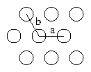
|
(b)
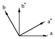
|
Figure 4:
(a) The Pt(111) surface with surface lattice vectors
,
, which are perpendicular to
=
(111).
(b) Reciprocal lattice vectors corresponding to the unit cell chosen
in (a);
and
subtend 60
and are
perpendicular to
.
From the convention (3.64) that
,
is orthogonal to
and
,
and
is orthogonal to
and
. So
and
must point in the directions indicated in
figure 5.4b. These vectors subtend 60
and generate a triangular lattice. The reciprocal-space lattice sites are
indexed in figure 5.6. Although this figure
appears superficially identical to figure 5.5, the
indexing is different due to the different angles subtended by the
basis vectors. From this point on, Bragg peaks are indexed using these
hexagonal units.
The conversion from cubic to hexagonal units is easily accomplished.
Writing both
-vectors as column vectors, then the matrix product
and
.
These transformation matrices are
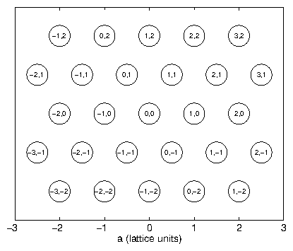
Figure 5: Indexing of surface units in real space.
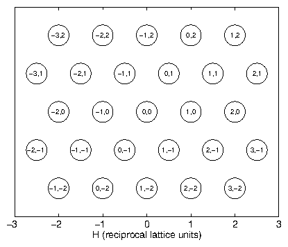
Figure 6: Indexing of surface units in reciprocal space.
4 Discussion of Incommensurate Structure
Tidswell and coworkers [131] have characterized the incommensurate bilayer that is present for intermediate potentials. They found a triangular array of x-ray scattering rods, sharp in and but diffuse in . The in-plane spacing was approximately 0.765 that of the truncation rods from the underlying platinum crystal. This corresponds to an in-plane bilayer lattice spacing 30% greater than Pt(111). Based upon their measurements of the positions and intensities of these scattering rods, they propose the model shown in figure 5.7. The Cu and Cl form a bilayer wherein the Cu atoms (small gray circles) are close to the Pt surface (large gray circles), and the Cl atoms (large empty circles) rest above the Cu, coordinated in the three-fold hollow sites of the hexagonal Cu lattice. If the Cl atoms are partially ionized toward Cl (making them larger), it is reasonable to assume that they are in close proximity to one another and determine the incommensurate lattice spacing. Tidswell et al. claim that the spacing is near to that of close-packed spheres with the Cl ionic radius.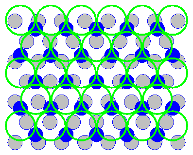
Figure 7:
Real-space map of the incommensurate overlayer, looking down on the
Pt (111) surface (gray). The Cu atoms (black) lie above the Pt substrate
and
are incommensurate with it. The Cl ions (hollow) lie in three-fold
hollow sites above the Cu layer.
It is surprising that the bilayer structure fails to follow the commensurate
lattice spacing, yet preserves the orientation of the underlying Pt lattice.
However, this scenario has been predicted by Novaco and McTague
[103]. They hypothesize static-distortion waves (analogous to
charge-density waves) in cases where the adlayer is weakly adsorbed to the
substrate. Minimizing the energy leads to a preferred orientation of the
adlayer with respect to the substrate. The relative orientation angle need
not be zero. Shaw, Fain, and Chinn [122] experimentally observed Ar
monolayers adsorbed onto graphite substrates at a range of low temperatures
(32 - 52 K). Their LEED (low-energy electron diffraction) measurements
demonstrated the relative orientation angle was inversely related to the Ar
monolayer lattice spacing. Their previous measurements with other adsorbed
noble gases find cases where the relative orientation is zero, as in our case.
A complete review on this subject can be found in the Pokrovsky and Talapov
[110].
Ben Ocko and coworkers
[104]
have studied a commensurate-incommensurate phase
transition in Br UPD on Au(100). Their results are compared with theoretical
predictions by Pokrovsky and Talapov
[109].
Our interest is primarily in the kinetics of this system, rather than
performing more detailed crystallography on the static phases. Therefore, it
is necessary to find a useful parameter to monitor the emergence of order
during formation of the bilayer. We chose the (0.765 0
) rod, because it
is the lowest index peak. Our choice of
depends upon two factors:
the minimization of background scattering from solution and polypropylene
film, and the
-dependent scattering from the bilayer itself. Absorption
effects (section 4.3.4) are most prominent for low
, as is the diffuse background scattering. The bilayer scattering
oscillates with
, as can be seen from examining the structure factor.
As mentioned above, the scattering is diffuse along the
axis. This is a
consequence of the nearly two-dimensional nature of the adsorbed layer.
However, the spacing between the Cu and Cl layers causes an interference
effect that is manifested in the oscillating intensity along
. A single
two-dimensional layer of hexagonally arranged atoms has a six-fold rotation
axis about the surface normal. Add a second commensurate layer with the same
number of atoms, by putting a chloride atom at position
for every
copper lattice position
. Assuming that these chlorides are attracted to
the copper layer, they will probably sit in the three-fold hollow sites
between copper atoms.
At this point, the symmetry is broken and the bilayer is only three-fold
symmetric.
To derive the structure factor, we need to find the coordinates of the
three-fold hollow site. Consider the location of the three-fold hollow site
between (0,0), (1,0), and (1,1). Referring to
figure 5.8, and recalling that the center of an
equilateral triangle is
of the distance from a side to the opposite
vertex, the position is
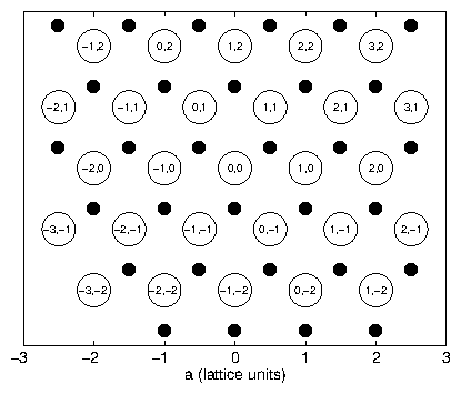
Figure 8: Real space image of bilayer. The open circles represent the
positions of the copper atoms, and the closed circles represent the
positions of the chloride atoms. In reality, the chloride atoms occupy
considerably more space than the copper atoms, as shown in
figure 5.7.
Now we turn our attention to the phase factors that influence the structure
factor of the bilayer. We can consider the two-dimensional CuCl bilayer as
though it were in isolation. The underlying Pt lattice has no fixed
periodicity with respect to it, and so will not change any of the structure
factors except at the specular condition
. As shown in
section 3.9.2, the structure factor due to the
addition of another atom is
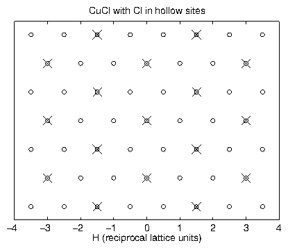
Figure 9: Reciprocal space map of monolayer (circles) and bilayer (crosses).
The monolayer points correspond to figure 5.6.
The bilayer points incorporate the
structure factor
from (5.17).
Now consider the
scattering.
Due to the three-fold symmetry,
the points
,
, and
illustrate all of the
possible cases. (The
is equivalent to
the
.)
These structure factors are plotted in figure 5.10.
As expected, they follow a simple sinusoidal form, but the initial phase at
is determined by (5.17).
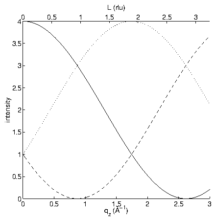
Figure 10: Structure factors for various the
(solid),
(dotted), and
(dashed) rods as a function of
.
The careful reader will note that I have neglected the atomic form factors of
Cu and Cl (that depend upon the ionization state, which is not known), and
the "Debye-Waller" factors due to disorder within the Cu-Cl bilayer.
However, in my opinion, there is a larger uncertainty that makes these
considerations moot. The illustration in figure 5.9 is only
one of two possibilities. The six-fold symmetry was broken by the assumption
that the chloride atoms fall into the upward-pointing triangles of
figure 5.5. We can equally well imagine that the
chloride atoms fall into the downward-pointing triangles. This is equivalent
to just a 60
rotation and changes the structure factors accordingly.
The three-fold hollow site immediately above (along the y-axis) from the
origin in figure 5.9 is
. (This is not
shown in the figure, because we previously took the other choice.) The
resulting structure factor is
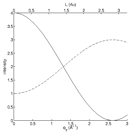
Figure 11: Structure factors for various the
(solid),
(dotted), and
(dashed) rods as a function of
.
The
and
coincide.
5 Static X-ray Data
Because of the conflicting reports of the CuCl overlayer structure at intermediate voltages, our first task was to make some static x-ray measurements. We have observed the overlayer structure numerous times during several experimental runs. Despite many attempts, we have never found scattering at the rods that can be attributed to the incommensurate overlayer, where and are integers up to 6. On the other hand, we have found scattering at the and rods that was voltage-dependent. This indicates that the measurements of Tidswell et al. [131] are correct, while the LEED measurements of Kolb [102] cannot be confirmed. Assuming that the seen in the LEED corresponds to the peak, then the additional peaks may be the result of multiple electron scattering. Alternatively, the ex situ experiment may change the ordering of the CuCl overlayer. This would not be surprising, as the vacuum and solution environments are very different. Figure 5.12 shows the overlayer Bragg peak at two different values of the applied potential. These data clearly demonstrate the presence of the incommensurate overlayer at 350 mV and its absence at 250 mV. The potential-independent background is due to scattering from the solution layer and the polypropylene film that contains it. By integrating for several seconds per -point, the signal can be easily resolved above this background. In the time-resolved measurements (chapter 6), where the x-ray signal is split into many time bins, this poses a considerable experimental challenge.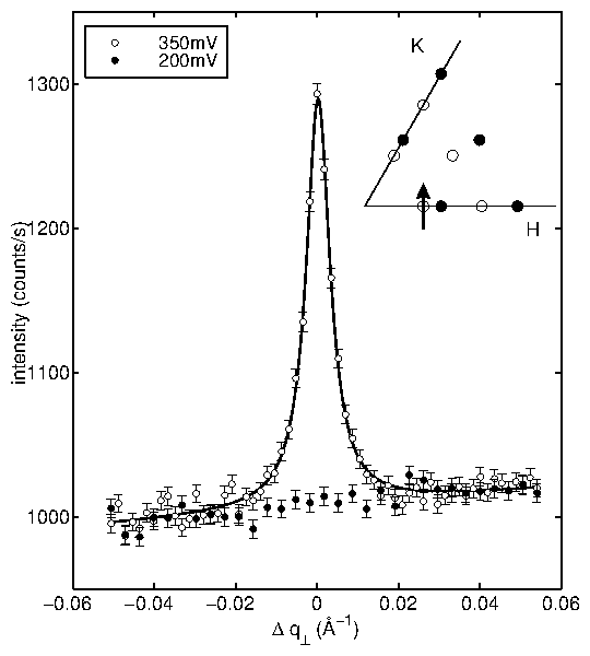
Figure 12:
Scattered intensity at
at 350 mV (hollow) and 200 mV (filled) vs. Ag/AgCl.
The solid line is the best fit to a Lorentzian line shape.
The shape of the diffraction peak is well-fit by a
Lorentzian line shape (the solid line in figure 5.12),
and the half-width at half-maximum
corresponds to a correlation
length
Å.
A Lorentzian is appropriate for systems with only
short range positional order.
The inset indicates the location of the Bragg rods of the two-dimensional
incommensurate overlayer (hollow) and the crystal truncation rods
(section 3.11.1) of the Pt substrate (filled).
The arrow represents the transverse scan shown in
the main figure. The transverse direction is denoted by
and is orthogonal to
and at constant
.
The corresponding x-ray scans through the overlayer Bragg peak, but along the
radial direction, are shown in
figure 5.13.
The radial direction is denoted by
and holds
and
constant.
In this case, the peak is broader than
scans through the
direction.
At first glance, this appears to indicate that the correlation function is
strongly asymmetric, with
.
This would be a surprising result.
However, as the next paragraphs will show, this can be accounted for by the
asymmetry of the resolution function.
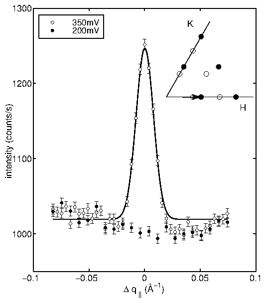
Figure 13:
Scattered intensity at
at 350 mV (hollow) and 200 mV (solid) vs. Ag/AgCl.
The solid line is the best fit to a Lorentzian line shape.
The asymmetry of the resolution is due to the differing longitudinal and
transverse resolutions.
Figure 5.14 depicts the elements of the scattering
geometry that determine the resolution.
A variation in
, the scattering angle between
and
, causes
to trace out the
major axis of the resolution ellipse. A variation in the magnitudes
and
, due to a variation in the
striking the
monochromator, causes
to trace out the
minor axis of the resolution ellipse.
As shown in the figure, the
longitudinal
and transverse
directions are not exactly coincident with the major and minor axes of the
resolution ellipse, but are rotated by
with respect to it.
A careful consideration of the resolution function is required for extremely
high-resolution experiments
[45].
For this relatively low-resolution experiment, the relative
rotation is neglected.
As already used, "perpendicular" (
) and "parallel"
(
) refer to vectors in the
,
plane (constant
). The term "longitudinal" refers a
direction along the scattering vector
, while "transverse" is
the direction orthogonal to this, but still in the scattering plane.
At this point in reciprocal space, the
direction
corresponds to the transverse direction.
The
direction corresponds closely to the longitudinal
direction, but is slightly different because of the constraint that
remain
constant in
.
The longitudinal resolution is found by
differentiating the definition of
(3.30),
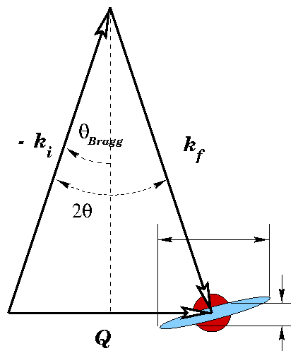
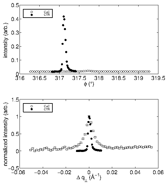
Figure 15:
Comparison of the
crystal truncation rod (filled) and the
overlayer Bragg scattering rod (hollow) at
.
Both are measured in the
direction and at
350 mV.
The overlayer peak is barely visible near
.
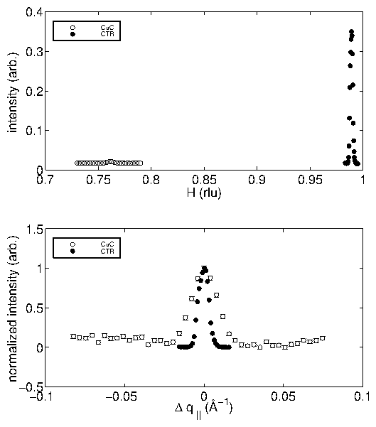
Figure 16:
Comparison of the
crystal truncation rod (filled) and the
overlayer Bragg scattering rod (hollow) at
.
Both are measured in the
direction and at
350 mV.
The calculated resolutions and measured peak widths are summarized in
table 5.1.
Each quoted value is a full-width at half-maximum.
The first and third columns are calculated longitudinal (5.19) and transverse (5.20)
resolutions for the CTR and overlayer rod. The second and fourth columns are
measured widths of peaks in the shown in the previous figures
for the
,
and
,
directions.
It may seem surprising that the measured width
for the CTR is
less than the calculated resolution
. However, this is just an
indication that
is not collinear with
the longitudinal direction.
Referring to figure 5.14, a cut through the
resolution ellipse along a direction other than the major axis (the
longitudinal direction) will always produce a more narrow profile.
Table 1:
Summary of measured peak widths (
,
)
and calculated resolutions (
,
).
All values are full-width at half-maxima.
| peak | (Å ) | (Å ) | (Å ) | (Å ) |
| Pt(111) CTR | ||||
| CuCl overlayer |
Chapter 6
Kinetic Measurements
1 Introduction
In this chapter, simultaneous electrochemical and x-ray scattering measurements of the ordering kinetics of the Cu-Cl bilayer during the transition from the commensurate copper overlayer to the incommensurate bilayer are reported. First, the time-resolved data are presented. Then, a simple theory for the nucleation of the incommensurate phase is described. The subsequent section presents data to support this model. Next, the entire - data set is presented, followed by a theory to describe it. The data is analyzed in the context of this theory, and excellent agreement is found. The final sections concern alternate models and further theoretical explanations.2 Time-Resolved Data
To observe the ordering kinetics during stripping, we employed a simple signal averaging technique. An example of the square-wave potential cycle that we applied is shown in figure 6.1a. At , the potential begins at 200 mV. The voltage is stepped to 350 mV at seconds. At seconds, the voltage is stepped back to 200 mV. This cycle repeats with a period of 40 seconds. Throughout this cycle, we simultaneously monitor both the current (figure 6.1b) and the intensity of the scattered x-rays at corresponding to the peak of figure 5.12. As expected, the incommensurate scattering peak is present only for values of the potential within the incommensurate phase. Note that the rise in the intensity of the scattered x-rays in figure 6.1c is much slower than the corresponding current transient in figure 6.1b. In contrast, the scattered intensity falls on a time scale similar to that of the current transient.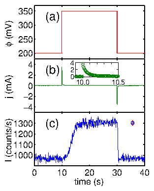
Figure 1:
(a) Applied potential steps.
(b) Current transients.
(c) Time dependence of the integrated intensity of
the
overlayer diffraction peak.
The current transients describe the
charge transfer at the electrode interface. These are due to two
contributing processes: the capacitive charging of the double-layer, and the
Faradaic charge transfer due to desorption/adsorption of ions.
Some previous chronoamperometric studies of closely related systems
[79,80]
exhibit distinct features in the current response that have been interpreted
as evidence of nucleation. These characteristic features are not present in
our data. We suspect that the geometry of the thin solution layer x-ray cell
may be responsible for this difference. The capacitive effect is greater for
our larger samples. This strong signal tends to mask other early features in
the current response. Also, in our apparatus, as compared with hanging
meniscus cells used in the other experiments, diffusion is comparatively
insignificant. First, diffusion from the "bulk" solution is not a
consideration for us, because the solution layer is so thin. Second, any
diffusion that does take place will occur in one dimension, rather than three.
Above the planar electrode face, the solution layer forms a very short
cylinder. The ions are in close proximity to the surface and conditions are
probably relatively uniform across the face, so diffusion is primarily along
the surface normal.
After numerous attempts, we can definitely say that there are no features in
the current response at the same time as the x-ray response. So
the measured current response is ascribed to desorption/deposition into a
disordered state (accompanied by charge transfer) which then gives rise to the
nucleation and growth of the equilibrium ordered phase. The rise in x-ray
intensity corresponds to an increased population in the incommensurate ordered
phase. The desorption process can be separated from the ordering process due
to the widely disparate time scales involved. Based on these data, we
hypothesize a scenario wherein the abrupt positive voltage step causes a
expulsion of some of the adsorbed copper ions. The remaining disordered ions
gradually reorganize into a two-dimensional crystalline state with a larger
lattice constant, incommensurate with the platinum substrate.
3 Stochastically Nucleated Islands
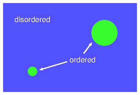
Figure 2: Cartoon of a nucleation process.
Consider the nucleation of (ordered) islands from a disordered phase,
as depicted in figure 6.2.
As usual, we define the Gibbs free energy of an island to be proportional to
the (electro)chemical potential and to the number of particles that comprise
the island. An island in contact with another phase will give rise to an
excess free energy term proportional to the surface area of contact. So the
existence of an island with
particles will lead to an excess of free
energy
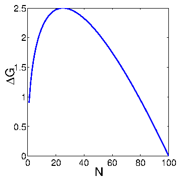
Figure 3: Example of Gibbs free energy
as a function of particle
number
.
For an arbitrary (perhaps fractal) island of dimensionality
, then
4 Instantaneous vs. Progressive Nucleation
Let be the number of nuclei at time . Following Schmickler, we assume "first-order kinetics" as follows: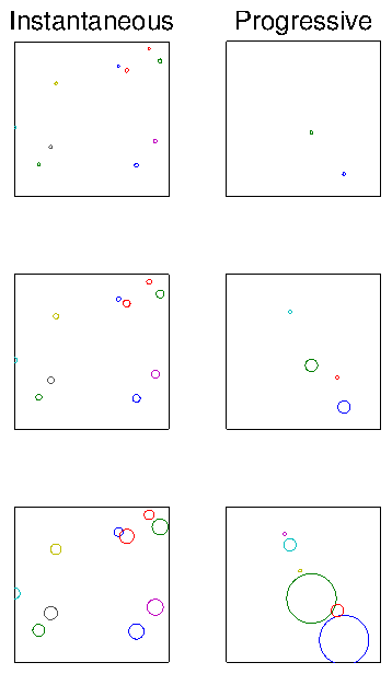
Figure 4: Cartoon contrasting progressive and instantaneous nucleation.
5 Characteristic Nucleation Time
Thus, we expect that as we quench deeper and deeper into the incommensurate phase, the transition will occur ever more rapidly. To test this hypothesis, we performed a series of voltage step measurements in which the applied potential was stepped from 200 mV (within the commensurate phase) to varying potentials within the incommensurate phase. As in the previous measurement, we measured the scattered intensity at the incommensurate overlayer peak position as a function of time. This corresponds to a series of experiments similar to the one shown in figure 6.1, but varying the value of the more positive voltage. This is shown in figure 6.5.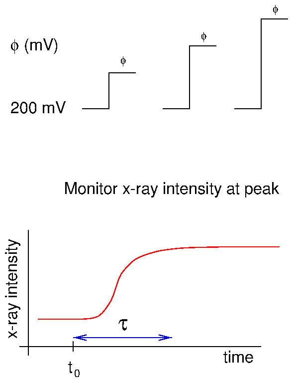
Figure 5: Diagram of voltage-quench experiments.
We characterized the resulting transition time by fitting the x-ray intensity
profiles (which resemble figure 6.1c) to a trapezoidal
functional form, as shown in figure 6.6. While this model
describes the data quite well, we ascribe no profound significance to it.
Rather, we use it simply to define a characteristic time,
, which should
be inversely proportional to
. The inset to figure 6.7
plots the resulting
values. The characteristic time scale describing
the ordering of the bilayer ranges varies from 50 seconds for shallow quenches
to 0.7 seconds for deep ones. Figure 6.7 illustrates the
exponential dependence of
on
. This fits Eq. (6.6)
with
, over the entire phase region. The linear slope demonstrates that
the growing islands are intrinsically two-dimensional (rather than
three-dimensional mounds or pits on the surface) and that these islands are
compact rather than fractal. The broad range of
also implies that our
two-dimensional cell geometry has not inhibited the nucleation processes, but
is only limited by the accessible range of voltage values. Furthermore, in
all cases,
is longer than the current transient indicating that
capacitive charging effects are not dominating our results.
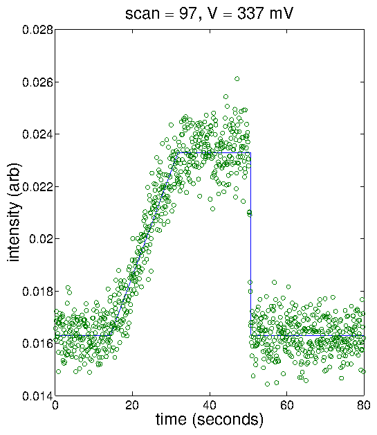
Figure 6: Typical trapezoidal fit
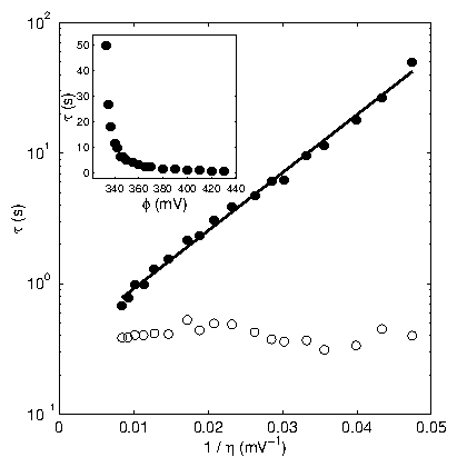
Figure 7: Characteristic rise time
vs. applied voltage.
Solid points represent x-ray transition times, while hollow points
represent the time scale for the desorption current transient to fall to
5% of its peak value. The straight line is a fit to the nucleation
model (6.8) with
. Inset:
on linear scale.
6 - Data
Now we turn our attention to the development of order in the incommensurate structure formed after desorption. In order to understand the kinetics of this ordering process, we need to access the full - dependent x-ray scattering. We repeat the time-resolved measurement of figure 6.1 for a series of -points linearly spaced along the same direction as shown in figure 5.12. An example of such a measurement is shown in figure 6.8. The first thing to note is that the peak remains centered at a constant value of , ruling out the possibility that the overlayer simply shifts its periodicity in response to the change in potential.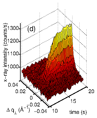
Figure 8:
Scattered intensity as a function of time
and transverse
scattering vector,
, with a false
gray-scale indicating intensity. Time bins have been merged for clarity.
From the discussion in section 5.5, the correlation
length is obtained from the width of the
diffraction peak and is believed to be determined by the finite size of
growing islands of Cu-Cl. The diffraction peak narrows with time, indicating
that these islands are growing. The total coverage is proportional to the
integrated intensity.
Ideally, we would collect a
-
data set for each
voltage
transition. However, the single data set shown in
figure 6.8 consumed 29 hours of synchrotron beam time.
With our constraints, it was not feasible to consider collecting many data
sets during that beam time allocation.
Because x-ray intensities obey Poisson counting statistics, for a
measured signal intensity
, the standard
deviation is
. As seen in figure 6.8, the
maximum signal in 1300 counts/second, while the
background is 1000 counts/second.
Because of this high background, we must count for long periods of time
to resolve the signal.
7 Growth of Two-Dimensional Islands
Up to now, we have discussed the number of islands, but not the total volume comprising this phase. As shown in section 6.5, the islands are intrinsically two-dimensional. This is not intuitively pleasing, since the bilayer itself is two-dimensional. Anticipating this result, in this section we will limit ourselves to the case of two-dimensional islands. Assume that each island grows by the incorporation of atoms into its boundary, and that this is the rate-limiting step for island growth. Then, for an island of atoms and radius , . This defines , the rate constant for individual island growth, which has units of [length time] . The area of the island is simply . Since (for a circular island) we have , we have two expressions for :8 Avrami Theorem
Following Avrami [14,15,16] consider a brief example of an area with circular islands, each of area . The extended coverage is . Of course, if the circles are placed randomly, then they will overlap somewhat and the true coverage will be less than the extended coverage . While the true coverage is bounded by the limits (no coverage) and (complete coverage), the extended coverage can be infinite. The probability that a particular point on the surface is not covered by a particular circle . So the probability that it is not covered by any of circles is . Assume that . Then in the limit and using , this probability becomes . Finally, the probability that a point is covered (which is just the "coverage" ) is9 Extended Coverage
In this section, I combine results from sections 6.7 and 6.8 to derive some simple expressions for the extended coverage. In general,10 Analysis of - Data
To begin the analysis of the data in figure 6.8, we fit each time slice to a Lorentzian line shape. A Lorentzian is the lowest order approximation to the structure factor for any system with only short range positional order. Some representative time slices and fits are shown by the thin lines in figure 6.9. From these fits, we extract the half-width at half-maximum ( ) and integrated intensity vs. time. These are shown as circles in figure 6.10b. As expected for growing islands, decreases with time. At the same time, the integrated intensity (proportional to the coverage) grows monotonically.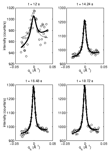
Figure 9:
Fits of data in figure 6.8 at representative times
12, 14.24, 16.48, and 18.72 seconds.
The thin lines
are from fits to the individual slices,
while the thick lines
are from the fit to (6.23).
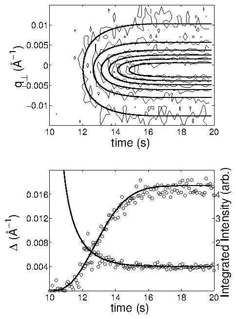
Figure 10:
(a) Contours of constant intensity of the data set (thin lines) in
figure 6.8 and from the best fit to (6.23)
(thick lines). (b) Best fit results for the half-width at half-maximum
(
; descending) and the integrated intensity (
; ascending)
vs. time. Circles are for separate Lorentzian fits to each
time slice and the
solid lines are from a fit to (6.23).
We can continue our analysis by incorporating the simple nucleation
and growth model considered previously.
Instead of fitting each time-slice independently, we now
want to fit the entire data set from figure 6.8
with a simple function of
few parameters.
This intensity function
we choose should satisfy the
following conditions.
First,
has a Lorentzian line shape
at any fixed time
.
This Lorentzian function is written
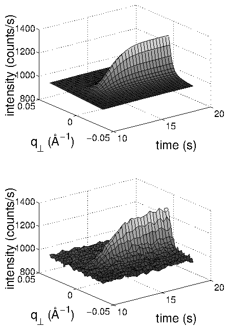
Figure 11: Comparison of (top) intensity generated from a fit
to (6.23)
with (bottom) measured x-ray intensity; time bins have been merged for
clarity.
All of the fit parameters are shown in
table 6.1; the physically interesting
ones are summarized in the top portion.
The initial time
, against which
times
are measured, was allowed to
float above 10 seconds (when the voltage was stepped), but fit to
10 seconds. There seems to be no
time delay before the nucleation process begins.
The growth parameter
is a product of various
parameters from (6.21)
that cannot be separated. The saturation island number
is
likewise coupled with a proportionality factor that cannot be isolated.
From the uncertainties
shown in the table,
all of the fit parameters are well-determined except for
, to which the
fit is relatively
insensitive.
This is an indication that either the data at early times (when there is very
low signal) is insufficient to fix this parameter, or that the observations
are in
the instantaneous limit (6.15),
where
does not depend on
.
Table 1: Parameters obtained from fits to figure 6.8.
The physically interesting parameters are shown in the top portion, and the
remainder are shown in the bottom portion.
| parameter | variable | fit value | units |
| initial time | s | ||
| growth parameter | Å s | ||
| saturation island number | Å | ||
| nucleation rate constant | s | ||
| peak intensity coefficient | arbitrary | ||
| peak position | Å | ||
| background constant | counts s | ||
| background slope | Å counts s | ||
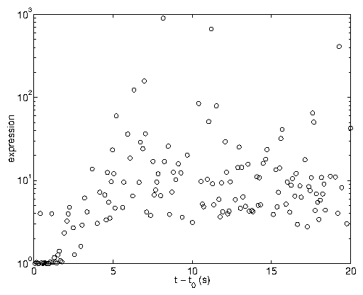
Figure 12: Plot of the expression on the right-hand side of (6.25)
vs.
. The noise in the
-values are primarily due to the
uncertainty in
, and make a test of (6.25)
impossible.
11 Density-Driven Nucleation and Growth Kinetics
Previously, we posited a voltage-dependent Gibbs free energy (6.6). For the case of two-dimensional circular clusters,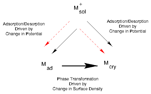
Figure 13:
Schematic of two possible deposition processes. The solid lines represent
mass flow (particle transfer) and dotted lines represent
current flow (charge transfer).
Upon the formation of a circular cluster with radius
,
the Gibbs free energy of the system changes by
.
has contributions from the difference of
chemical potentials of the lattice phase
and disordered adsorbed phase
and from the surface energy.
12 Step Chronoamperometry of an Ideal System
In section 2.5.2, we considered the electrode to be a perfect sink for ions: any ions that arrive at are deposited onto the electrode irreversibly. This is the meaning of the boundary condition (2.45)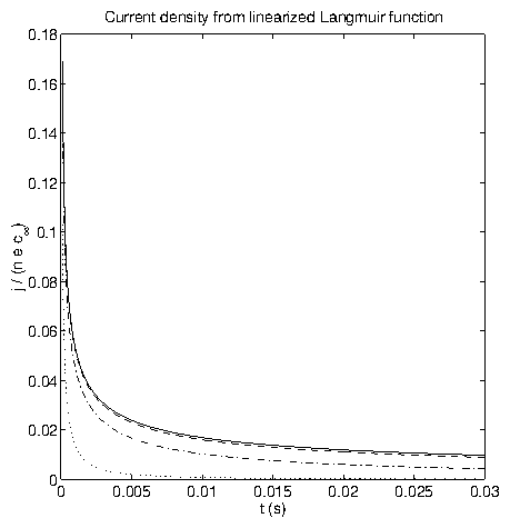
Figure 14: Current density at the electrode surface
from (6.48) with
(dotted),
(dot-dashed), and
(dashed). Note that
is nearly
indistinguishable from the Cottrell result (solid). I have chosen
, which is typical of aqueous
solutions.
13 Discussion
The basic scenario is that the applied potential step drives copper off of the surface and the Cu-Cl grains then nucleate and grow. Upon reversal of the potential step, the Cu-Cl bilayer is destroyed as the commensurate copper layer is formed. From the exponential dependence of the time scale on voltage (figure 6.7), it is now clear why Cu/Cl/Pt(111) cyclic voltammetry (figure 5.2) always shows hysteresis, even for extremely slow sweep rates. Incorporating the nucleation and growth model into the cyclic voltammetry formula should lead to quantitative predictions for the degree of hysteresis as a function of sweep rate. However, it is unlikely that cyclic voltammetry alone would provide sufficient evidence for nucleation and growth; there are many processes that can affect electrode kinetics and cause similar responses. Instead, electrochemists typically study nucleation with chronoamperometry [79,80]. We have carefully considered possible effects of the thin solution layer on the ordering kinetics after a potential step. If the thin-layer were an inhibiting factor, we would expect to find an upper limit to the rate at which the nucleation process could take place. This is not apparent in our data. As shown in figure 6.7, the fastest observable time scale is limited by the constraint that the voltage quench not reach into phase A, beyond the incommensurate phase B. Furthermore, there is no evidence of any roll-over in the voltage dependence of the ordering time constant. Finally, the ordering time constant is always longer than the electronic time constant. In standard deposition-nucleation problems [117], the voltage dependence in the Gibbs free energy (6.3) is a result of the differing electric potentials in the bulk solution and at the surface of the electrode. In our problem, the incommensurate and commensurate phases are both near the electrode surface. The charge transfer from the platinum surface precedes the ordering and may be voltage dependent. In particular, how much of the charge is shared between the Cu and Cl atoms is unknown. It has been shown that the ionization state does not jump directly from Cu to Cu [78,4]. Another possibility is that the Cu or Cl ions change their positions (especially along the direction) as a precursor to desorption out of the ordered state. Expanded or compressed layers, which are voltage-controlled, have been observed in several UPD systems. To resolve these underlying issues, more data on this transition must be acquired. Time-resolved in situ reflectivity, both specular and non-specular, would help to clarify the positions and occupancies of the Cu and Cl layers throughout the desorption process. X-ray standing waves, which have been applied to UPD [5,35,3], are particularly sensitive to the positions of ordered layers above the electrode surface. It may also be helpful to take data on a related UPD process: Cu on Au(111) in H SO [133]. This one of the most studied systems and has been extremely well-characterized. The gold surface is much easier to work with and does not oxidize as readily as platinum, simplifying the sample transfer (section 4.3.7) and subsequent data acquisition. Scattering from the commensurate overlayer occurs at the same , positions as the Pt(111) crystal truncation rods and will be difficult to observe. Thus, experimental information on the reverse reaction, formation of the commensurate layer, will be difficult to obtain. Finally, a comparison of the electrochemical current transients in the hanging-meniscus cell and the x-ray cell is necessary. Hanging-meniscus data show distinct nucleation bumps that are absent in the x-ray cell. While capacitive charging effects (which are enhanced in the x-ray cell) may mask some features, a systematic study of each would resolve the discrepancy and clarify the voltage dependence in (6.3).
Chapter 7
Conclusions
In conclusion, we have studied a system wherein desorption (rather than
deposition) is followed by ordering. The charge-transfer process is much
faster than the development of long-range order. The x-ray data are well
described by a nucleation and growth model with only a few parameters. The
potential-step experiments demonstrate that the rate of ordering agrees well
with nucleation models over two decades in time, and is not limited by the
thin-layer geometry.
Electrochemistry is a good model system for studying growth phenomena in
general. In comparison with in vacuo systems, it has the advantage
that
heteroepitaxial material can be removed to recover the initial substrate. So
the same deposition (or desorption) processes can be studied repeatedly, under
identical conditions, and without having to change samples. Also,
electrochemical systems can be simpler, and components are less expensive,
than for ultra-high vacuum systems. This is more practical for traveling to
distant locations (such as synchrotrons).
Despite the "conventional wisdom", it is possible to perform good kinetic
x-ray measurements in a thin-layer electrochemical cell. The limiting rates
are not specifically constrained by the cell itself. Voltammograms of ideal
quality are a necessary condition to detecting the x-ray signal. Crystal
quality is a determining factor in both voltammetry and the bilayer x-ray
scattering. To this end, we developed a polishing / annealing procedure and
apparatus that have now propagated to other research groups in Clark Hall.
We have simultaneously measured in situ x-ray scattering
from the adsorbed incommensurate bilayer and current transients. This allows
us to directly address the kinetics of the nonequilibrium desorption/ordering
process. Upon a positive voltage step, there is Cu desorption, and the
commensurate structure transforms into an incommensurate structure, with a
larger in-plane lattice constant. During this process, we see a current
transient and the emergence of an x-ray scattering peak. The current
transients have two components: the capacitive charging of the double-layer,
and the Faradaic charge transfer due to desorption/adsorption of ions. We
have not yet been able to separate the two. The x-ray scattering intensity
indicates the ordering of the incommensurate bilayer. The rise in integrated
intensity is proportional to the increasing number density in the ordered
phase. The narrowing of the peak corresponds to a increasing correlation
length, which implies growing phase domains.
Using a nucleation and growth model, we can fit the entire
-
data set
(
points) to a function of a few variables.
Extending these arguments, we demonstrate that the ordering time scales with
voltage over the entire range, in quantitative agreement with the nucleation
and growth of two-dimensional islands.
All we know about the desorption process is contained in the
current transient data.
One could better determine when the copper ions leave the surface by
performing a similar kinetic x-ray experiment but monitoring the specular
reflectivity instead of the intensity of the Cu-Cl order parameter.
The information gained would be very interesting; however,
the experiment would be a major undertaking, requiring a different
cell design and many months of experimenting.
Furthermore, the results would not affect the conclusions of the
current experiment.
Rather, they might shed some light on what happens before the nucleation
and growth process begins.
Further studies could explore the relationship between
geometry-dependent diffusion processes, charge transfer at the interface, and
nucleation mechanisms.
Some future experimental directions have already been detailed in
section 4.6. Additional chronoamperometric
measurements in a cell where the thickness of the solution layer could be
systematically varied would allow one to investigate whether the desorption
process is diffusion-limited in one limit and reaction-rate-limited in the
other. These measurements are also well beyond the scope of the current
investigation, requiring new experimental cells and, again, the results would
not affect our current conclusions.
Appendix 1
Gaussian Distributions
This appendix summarizes some relevant results on Gaussian distributions for
the reader who may not be familiar with them.
Consider the cumulant expansion [70] for
, where
is considered small.
Here, we will only expand to second order, though the extension to higher
orders is straightforward.
To derive the cumulant expansion,
begin with
Now, the expectation value of is
For a Gaussian distribution, all of the terms of the cumulant expansion beyond second order are identically zero. For this reason, the assumption of a Gaussian distribution is equivalent to the assumption that is sufficiently small (so that terms beyond second order can be neglected). I mention one more useful relation, used in section 3.10. Assuming that the Gaussian approximation is valid and ,
Appendix 2
Diffusion Equation
This treatment expands upon the three-dimensional treatment by McQuarrie
[99] and extends it to arbitrary dimensionality.
McQuarrie actually suggests two ways to give the
result (B.14); I am using the first.
The diffusion equation for
is
Take the case,
References
- [1]
- Henke Atomic Scattering Factors. http://xray.uu.se/hypertext/henke.html. Other x-ray data is available at http://xray.uu.se.
- [2]
- NIST Physical Reference Data. http://physics.nist.gov/PhysRefData/contents.html. Paper version is [53].
- [3]
- H. D. Abruna, G. M. Bommarito, and D. Acevedo. The study of solid/liquid interfaces with X-ray standing waves. Science, 250(4977):69-74, October 1990.
- [4]
- H. D. Abruña, J. M. Feliu, J. D. Brock, L. J. Buller, E. Herrero, J. Li, R. Gómez, and A. Finnefrock. Anion and electrode surface structure effects on the deposition of metal monolayers: Electrochemical and time-resolved surface diffraction studies. Electrochimica Acta, 43(19-20):2899-2909, 1998.
- [5]
- H. D. Abruna, J. H. White, G. M. Bommarito, M. J. Albarelli, D. Acevedo, and M. J. Bedzyk. Structural studies of electrochemical interfaces with X-rays. Rev. Sci. Instrum. (USA), 60(7):2529-32, July 1989.
- [6]
- R. Adzi\'c. In H. Gerisher and C. Tobias, editors, Advances in Electrochemistry and Electrochemical Engineering, volume 13, page 159. Wiley and Sons, New York, 1978.
- [7]
- R.R. Adzic. Electrocatalysis on surfaces modified by foreign metal adatoms. Israel Journal of Chemistry, 18(1):166-81, 1979.
- [8]
- Neil W. Ashcroft. Statistical mechanics. lecture notes, spring 1993.
- [9]
- Neil W. Ashcroft and N. David Mermin. Solid State Physics, page 100. In [13], 1976.
- [10]
- Neil W. Ashcroft and N. David Mermin. Solid State Physics, page 86. In [13], 1976.
- [11]
- Neil W. Ashcroft and N. David Mermin. Solid State Physics, chapter Appendix N. In [13], 1976.
- [12]
- Neil W. Ashcroft and N. David Mermin. Solid State Physics, page 794. In [13], 1976.
- [13]
- Neil W. Ashcroft and N. David Mermin. Solid State Physics. W.B. Saunders, 1976.
- [14]
- M. Avrami. Kinetics of phase change. i. J. Chem. Phys., 7:1103-1112, 1939.
- [15]
- M. Avrami. Kinetics of phase change. ii. J. Chem. Phys., 8:212-224, 1940.
- [16]
- M. Avrami. Kinetics of phase change. iii. J. Chem. Phys., 9:177-184, 1941.
- [17]
- A.-L. Barabási and H. E. Stanley. Fractal Concepts in Surface Growth. Cambridge University Press, Cambridge, 1995.
- [18]
- Allen J. Bard and Larry R. Faulkner. Electrochemical Methods: Fundamentals and Applications, page 9. In [24], 1980.
- [19]
- Allen J. Bard and Larry R. Faulkner. Electrochemical Methods: Fundamentals and Applications, page 505. In [24], 1980.
- [20]
- Allen J. Bard and Larry R. Faulkner. Electrochemical Methods: Fundamentals and Applications, page 510. In [24], 1980.
- [21]
- Allen J. Bard and Larry R. Faulkner. Electrochemical Methods: Fundamentals and Applications, page 563. In [24], 1980. Figure 13.4.2.
- [22]
- Allen J. Bard and Larry R. Faulkner. Electrochemical Methods: Fundamentals and Applications, page 60. In [24], 1980.
- [23]
- Allen J. Bard and Larry R. Faulkner. Electrochemical Methods: Fundamentals and Applications, pages 500-515. In [24], 1980.
- [24]
- Allen J. Bard and Larry R. Faulkner. Electrochemical Methods: Fundamentals and Applications. Wiley, 1980.
- [25]
- Allen J. Bard and Larry R. Faulkner. Electrochemical Methods: Fundamentals and Applications, pages 128-131. In [24], 1980.
- [26]
- Allen J. Bard and Larry R. Faulkner. Electrochemical Methods: Fundamentals and Applications, pages 121-127. In [24], 1980.
- [27]
- Allen J. Bard and Larry R. Faulkner. Electrochemical Methods: Fundamentals and Applications, page 51. In [24], 1980.
- [28]
- Allen J. Bard and Larry R. Faulkner. Electrochemical Methods: Fundamentals and Applications, pages 142-146. In [24], 1980.
- [29]
- Allen J. Bard and Larry R. Faulkner. Electrochemical Methods: Fundamentals and Applications, page 515. In [24], 1980.
- [30]
- Allen J. Bard and Larry R. Faulkner. Electrochemical Methods: Fundamentals and Applications, chapter 12.1. In [24], 1980.
- [31]
- Allen J. Bard and Larry R. Faulkner. Electrochemical Methods: Fundamentals and Applications, pages 521-523. In [24], 1980.
- [32]
- U. Bergmann, D.P. Siddons, and J.B. Hastings. Time-dependent polarization in Moessbauer experiments with synchrotron radiation. 2. Hyperfine Interact. (Switzerland), 92(1):1113-21, November 1994.
- [33]
- A. Bewick and B. Thomas. J. Electroanal. Chem., 70:239, 1976.
- [34]
- J. O'M. Bockris, M. A. Devanathan, and K. Müller. Proc. R. Soc., A274:55, 1963. Cited in Brett and Brett.
- [35]
- G. M. Bommarito, D. Acevedo, J. F. Rodriguez, and H. D. Abru na. In-Situ x-ray standing wave study of Cu UPD on an iodine covered surface. In J. Gordon and A. Davenport, editors, Symposium on X-ray Methods in Electrochemistry, page 125. The Electrochemical Society, Pennington, NJ, 1972.
- [36]
- Itamar Borukhov, David Andelman, and Henri Orland. Steric effects in electrolytes: A modified Poisson-Boltzmann equation. Phys. Rev. Lett., 79(3):435-438, July 1997.
- [37]
- R.N. Bracewell. The Fourier Transform and its Applications. McGraw-Hill, New York, 1986.
- [38]
- Christopher M.A. Brett and Ana Maria Oliveira Brett. Electrochemistry: Principles, Methods, and Applications, page 52. In [42], 1993.
- [39]
- Christopher M.A. Brett and Ana Maria Oliveira Brett. Electrochemistry: Principles, Methods, and Applications, pages 44-54. In [42], 1993.
- [40]
- Christopher M.A. Brett and Ana Maria Oliveira Brett. Electrochemistry: Principles, Methods, and Applications, pages 138-140. In [42], 1993.
- [41]
- Christopher M.A. Brett and Ana Maria Oliveira Brett. Electrochemistry: Principles, Methods, and Applications, pages 85-90. In [42], 1993.
- [42]
- Christopher M.A. Brett and Ana Maria Oliveira Brett. Electrochemistry: Principles, Methods, and Applications. Oxford Univ. Press, 1993.
- [43]
- Christopher M.A. Brett and Ana Maria Oliveira Brett. Electrochemistry: Principles, Methods, and Applications, page 22. In [42], 1993.
- [44]
- Christopher M.A. Brett and Ana Maria Oliveira Brett. Electrochemistry: Principles, Methods, and Applications, page 137. In [42], 1993.
- [45]
- J. D. Brock, A. C. Finnefrock, K. L. Ringland, and E. Sweetland. Detailed structure of a charge-density wave in a quenched random field. Phys. Rev. Lett., 73(26):3588-91, December 1994.
- [46]
- Joel D. Brock. X-ray Scattering Study of Bond Orientational Order in Liquid Crystal Films. PhD thesis, Massachusetts Institute of Technology, May 1987.
- [47]
- Joel D. Brock. X-ray Scattering Study of Bond Orientational Order in Liquid Crystal Films. PhD thesis, Massachusetts Institute of Technology, May 1987.
- [48]
- Joel D. Brock. Linearized langmuir nucleation model. Unpublished, 1997.
- [49]
- F. Brossard, V. H. Etgens, and A. Tadjeddine. In situ surface X-ray diffraction using a new electrochemical cell optimised for third generation synchrotron light sources. Nuclear Instruments and Methods in Physics Research B, 129:419-422, 1997.
- [50]
- Stanley Bruckenstein and Barry Miller. Unraveling reactions with rotating electrode. Accounts of Chemical Research, 10:54-61, 1977.
- [51]
- E. Budevski, G. Staikov, and W.J. Lorenz. Electrochemical Phase Formation and Growth: An Introduction to the Initial Stages of Metal Deposition. VCH Publ., Weinheim, 1996.
- [52]
- Lisa Jean Buller. Electrochemical and X-ray Studies of the Structure and Dynamics of Deposition of Metal Monolayers. PhD thesis, Cornell University, August 1997.
- [53]
- C. T. Chantler. J. Phys. Chem. Ref. Data, 24:71, 1995.
- [54]
- D. L. Chapman. Phil. Mag., 25:475, 1913. Cited in Brett and Brett.
- [55]
- Ruel Vance Churchill. Operational Mathematics. McGraw-Hill, New York, 1971. Cited in [48].
- [56]
- R. Coisson. X-ray sources. In M. Schlinker, M. Fink, J.P. Goedgebuer, C. Malgrange, J. Ch. Viénot, and R.H. Wade, editors, Imaging Processes and Coherence in Physics, pages 51-56. Springer-Verlag, Berlin, 1980.
- [57]
- B.D. Cullity. Elements of X-Ray Diffraction. Addison-Wesley, Reading, Massachusetts, second edition, 1978.
- [58]
- B.D. Cullity. Elements of X-Ray Diffraction, page 112. In [57], second edition, 1978.
- [59]
- B.D. Cullity. Elements of X-Ray Diffraction, page 392. In [57], second edition, 1978.
- [60]
- B.D. Cullity. Elements of X-Ray Diffraction, chapter Appendix 12. In [57], second edition, 1978.
- [61]
- B.D. Cullity. Elements of X-Ray Diffraction, pages 135-139. In [57], second edition, 1978.
- [62]
- B.D. Cullity. Elements of X-Ray Diffraction, page 14. In [57], second edition, 1978.
- [63]
- B.D. Cullity. Elements of X-Ray Diffraction, pages 135-139. In [57], second edition, 1978.
- [64]
- G.J. Edens, X. Gao, and M.J. Weaver. J. Electroanal. Chem., 375:357, 1994.
- [65]
- A. C. Finnefrock, L. J. Buller, K. L. Ringland, J. D. Brock, and H. D. Abruña. Time-resolved surface x-ray scattering study of surface ordering of electrodeposited layers. J. Amer. Chem. Soc., 119:11703-11704, December 1997.
- [66]
- A. C. Finnefrock, L. J. Buller, K. L. Ringland, P. D. Ting, H. D. Abruña, and J. D. Brock. Time-resolved measurements of overlayer ordering in electrodeposition. In P. C. Andricacos, S. G. Corcoran, J.-L. Delplancke, T. P. Moffat, and P. S. Searson, editors, Electrochemical Synthesis and Modification of Materials. Symposium, volume 451, pages 49-55. Materials Research Society, 1997.
- [67]
- Luigi Galvani. Commentary on the effect of electricity on muscular motion; a translation of Luigi Galvani's De viribus electricitatis in motu musculari commentarius. E. Licht, Cambridge, Mass., 1953. English translation.
- [68]
- Luigi Galvani. Opere scelte ... A cura di Gustavo Barbensi. Unione tipografico editrice torinese, Torino, Italy, 1967. Annotated copy of original. In Italian.
- [69]
- Doon Gibbs, B. M. Ocko, D. M. Zehner, and S. G. J. Mochrie. Absolute x-ray reflectivity study of the Au(100) surface. Phys. Rev. B, 38(11):7303-7310, 1988.
- [70]
- N. Goldenfeld. Lectures on Phase Transitions and the Renormalization Group, page 261. Addison-Wesley, 1992.
- [71]
- R. Gómez, J.M. Feliu, and H. D. Abruña. Langmuir, 10:4315, 1994.
- [72]
- R. Gómez, H. S. Yee, G. M. Bommarito, F. M. Feliu, and H. D. Abru na. Anion effects and the mechanism of Cu UPD on Pt(111): X-ray and electrochemical studies. Surf. Sci., 335:101, 1995.
- [73]
- G. Gouy. Compt. Rend., 149:654, 1910. Cited in Brett and Brett.
- [74]
- D. C. Grahame. Chem. Rev., 41:441, 1947. Cited in Brett and Brett.
- [75]
- G. Grübel, K. G. Huang, Doon Gibbs, D. M. Zehner, A. R. Sandy, and S. G. J. Mochrie. Phys. Rev. B, 48:18119, 1993.
- [76]
- T. Hachiya, H. Honbo, and K. Itaya. J. Electroanal. Chem., 315:275, 1991.
- [77]
- Herman and Winick, editors. Synchrotron Radiation Science: A Primer. World Scientific.
- [78]
- E. Herrero, L. J. Buller, J. Li, A. C. Finnefrock, A. B. Solomón, C. Alonso, J. D. Brock, and H.D . Abruña. Electrodeposition dynamics: Electrochemical and x-ray scattering studies. Electrochimica Acta, 44(6-7):983-992, 1998.
- [79]
- M. H. Hölzle, U. Retter, and D. M. Kolb. The kinetics of structural changes in Cu adlayers on Au(111). J. Electroanal. Chem., 371:101-109, 1994.
- [80]
- M. H. Hölzle, V. Zwing, and D. M. Kolb. The influence of steps on the deposition of Cu onto Au(111). Electrochim. Acta, 40(10):1237-1247, 1995.
- [81]
- J.D. Jackson. Classical Electrodynamics, page 516. In [83], second edition, 1975.
- [82]
- J.D. Jackson. Classical Electrodynamics, page 679. In [83], second edition, 1975.
- [83]
- J.D. Jackson. Classical Electrodynamics. John Wiley & Sons, New York, second edition, 1975.
- [84]
- J.D. Jackson. Classical Electrodynamics, pages 281-282. In [83], second edition, 1975.
- [85]
- J.D. Jackson. Classical Electrodynamics, pages 284-288. In [83], second edition, 1975.
- [86]
- M. Kardar, G. Parisi, and Y. Zhang. Dynamic scaling of growing interfaces. Phys. Rev. Lett., 56:889, 1986.
- [87]
- Kwang-Je Kim. Characteristics of synchrotron radiation. In Douglas Vaughn, editor, X-Ray Data Booklet, chapter 4. Lawrence Berkeley Laboratory, April 1986.
- [88]
- James B. Knight, Ashvin Vishwanath, James P. Brody, and Robert H. Austin. Hydrodynamic focusing on a silicon chip: Mixing nanoliters in microseconds. Phys. Rev. Lett., 80(17):3863-3866, April 1998.
- [89]
- D. Kolb. In H. Gerisher and C. Tobias, editors, Advances in Electrochemistry and Electrochemical Engineering, volume 11, page 125. Wiley and Sons, New York, 1978.
- [90]
- D. M. Kolb, A. Jaff-Golze, and M. S. Zei. Dechema Monographien, 102:53-64, 1986.
- [91]
- J. Li and H. D. Abruña. J. Phys. Chem., 101:244, 1997.
- [92]
- O.M. Magnussen, J. Hotlos, R.J. Nichols, D.M. Kolb, and R.J. Behm. Atomic structure of Cu adlayers on Au(100) and Au(111) electrodes observed by in situ scanning tunneling microscopy. Physical Review Letters, 64(24):2929-32, June 1990.
- [93]
- S. Manne, P.K. Hansma, J. Massie, V.B. Elings, and A.A. Gewirth. Science, 251:183, 1991.
- [94]
- N. Markovi\'c and P. N. Ross. Effect of anions on the underpotential deposition of Cu on Pt(111) and Pt(100) surfaces. Langmuir, 9(2):580-590, 1993.
- [95]
- H. Matsumoto, J. Inukai, and M. Ito. J. Electroanal. Chem., 379:223, 1994.
- [96]
- Donald A. McQuarrie. Statistical Mechanics, page 87. In [100], 1976.
- [97]
- Donald A. McQuarrie. Statistical Mechanics, chapter 20. In [100], 1976.
- [98]
- Donald A. McQuarrie. Statistical Mechanics, chapter 15. In [100], 1976.
- [99]
- Donald A. McQuarrie. Statistical Mechanics, pages 513-514. In [100], 1976.
- [100]
- Donald A. McQuarrie. Statistical Mechanics. Harper Collins, New York, NY, 1976.
- [101]
- O.R. Melroy, M.F. Toney, G.L. Borges, M.G. Samant, J.B. Kortright, P.N. Ross, and L. Blum. Phys. Rev. B, 38:10962, 1988.
- [102]
- R. Michaelis, M. S. Zei, R. S. Zhai, and D. M. Kolb. The effect of halides on the structure of copper underpotential-deposited onto Pt(111): a low-energy electron diffraction and X-ray photoelectron spectroscopy study. J. Electroanal. Chem., 339:299-310, 1992.
- [103]
- Anthony D. Novaco and John P. McTague. Orientational epitaxy - the orientational ordering of incommensurate structures. Phys. Rev. Lett., 38(22):1286, 1977.
- [104]
- B. M. Ocko, O. M. Magnussen, J. X. Wang, and Th. Wandlowski. One-dimensional commensurate-incommensurate transition: Bromide on the Au(100) electrode. Phys. Rev. B, 53(12):R7654-R7657, March 1996.
- [105]
- B. M. Ocko, J. X. Wang, and T. Wandlowski. Bromide adsorption on Ag(001): A potential induced two-dimensional Ising order-disorder transition. Phys. Rev. Lett., 79:1511-1514, August 1997.
- [106]
- B. M. Ocko, Jia Wang, Alison Davenport, and Hugh Isaacs. Phys. Rev. Lett., 65:1466, 1990.
- [107]
- B.M. Ocko, G.M. Watson, and J. Wang. J. Phys. Chem., 98:897, 1994.
- [108]
- J. M. Orts, R. Gómez, J. M. Feliu, A. Aldaz, and J. Clavilier. Electrochim. Acta, 39:1519, 1994.
- [109]
- V. L. Pokrovsky and A. L. Talapov. Phys. Rev. Lett., 42(66), 1979.
- [110]
- V. L. Pokrovsky and A. L. Talapov. Theory of Incommensurate Crystals, volume 1 of Soviet Scientific Reviews, Supplement Series Physics. Harwood Academic Publishers, New York, NY, 1984. translated by J. George Adashko.
- [111]
- I. K. Robinson. Crystal truncation rods and surface roughness. Phys. Rev. B, 33(6):3830, 1986.
- [112]
- J.J. Sakurai. Advanced Quantum Mechanics. Addison-Wesley, 1967.
- [113]
- M. G. Samant, M. F. Toney, G. L. Borges, L. Blum, and O. R. Melroy. Surf. Sci. Lett., 193:L29, 1988.
- [114]
- Wolfgang Schmickler. Interfacial Electrochemistry, page 1. In [117], 1996.
- [115]
- Wolfgang Schmickler. Interfacial Electrochemistry, pages 21-32. In [117], 1996.
- [116]
- Wolfgang Schmickler. Interfacial Electrochemistry, pages 33-34. In [117], 1996.
- [117]
- Wolfgang Schmickler. Interfacial Electrochemistry. Oxford University Press, New York, 1996.
- [118]
- Wolfgang Schmickler. Interfacial Electrochemistry, pages 17-20. In [117], 1996.
- [119]
- J. W. Schultze. Ber. Bunsenges. Phys. Chem., 74:705, 1970.
- [120]
- J. W. Schultze and K. J. Vetter. J. Electroanal. Chem., 44:63, 1973.
- [121]
- J.W. Schultze and D. Dickertmann. Surf. Sci., 54:489, 1976.
- [122]
- Christopher G. Shaw, S. C. Fain, Jr., and M. D. Chinn. Observation of orientational ordering of incommensurate argon monolayers on graphite. Phys. Rev. Lett., 41(14):955, 1978.
- [123]
- Z. Shi, S. Wu, and J. Lipkowski. Electrochim. Acta, 40:9, 1995.
- [124]
- S.K. Sinha, E.B. Sirota, S. Garoff, and H.B. Stanley. X-ray and neutron scattering from rough surfaces. Phys. Rev. B, 38:2297, 1988.
- [125]
- O. Stern. Z. Elektrochem., 30:508, 1924. Cited in Brett and Brett.
- [126]
- Mark Sutton. private communication.
- [127]
- E. Sweetland, A. C. Finnefrock, W. J. Podulka, M. Sutton, J. D. Brock, D. DiCarlo, and R. E. Thorne. X-ray-scattering measurements of the transient structure of a driven charge-density wave. Physical Review B (Condensed Matter), 50(12):8157-65, September 1994.
- [128]
- S. Szabó. Int. Rev. Phys. Chem., 10:207, 1991.
- [129]
- A. Tadjeddine, G. Tourillon, and D. Guay. Electochim. Acta, 36:1859, 1991.
- [130]
- Saul Teukolsky. Properties of synchrotron radiation. handout for Physics 561, Cornell University, 1992.
- [131]
- I. M. Tidswell, C. A. Lucas, N. M. Markovic, and P. N. Ross. Surface-structure determination using anomalous X-ray scattering: underpotential deposition of copper on Pt(111). Phys. Rev. B, 51(15):10205-8, April 1995.
- [132]
- M.F. Toney, J.G. Gordon, M.G. Samant, G.L. Borges, O. Melroy, L.-S. Kau, D.G. Wiesler, D. Yee, and L.B. Sorensen. Phys. Rev. B, 42:5594, 1990.
- [133]
- M.F. Toney, J.N. Howard, J. Richer, G.L. Borges, J.G. Gordon, O.R. Melroy, D. Yee, and L.B. Sorensen. Phys. Rev. Lett., 75:4772, 1995.
- [134]
- Richard D. Varjian. Electrolytic processing. Interface, 3(3):24-28, Fall 1994.
- [135]
- I. Villegas and J. L. Stickney. J. Electrochem. Soc., 138:1310, 1991.
- [136]
- I. Villegas and J. L. Stickney. J. Electrochem. Soc., 139:686, 1992.
- [137]
- H. L. F. von Helmholtz. Ann. Physik, 89:211, 1853. Cited in Brett and Brett.
- [138]
- H. L. F. von Helmholtz. Ann. Physik, 7:337, 1879. Cited in Brett and Brett.
- [139]
- J. Wang, A.J. Davenport, H.S. Isaacs, and B.M. Ocko. Science, 255:1416, 1992.
- [140]
- J. Wang, B.M. Ocko, A.J. Davenport, and H.S. Isaacs. Phys. Rev. B, 46:10321, 1992.
- [141]
- B.E. Warren. X-ray Diffraction, chapter 1. In [148], 1990.
- [142]
- B.E. Warren. X-ray Diffraction, pages 7-12. In [148], 1990.
- [143]
- B.E. Warren. X-ray Diffraction, chapter Appendix 4 and 5. In [148], 1990.
- [144]
- B.E. Warren. X-ray Diffraction, pages 331-332. In [148], 1990.
- [145]
- B.E. Warren. X-ray Diffraction, pages 35-38. In [148], 1990.
- [146]
- B.E. Warren. X-ray Diffraction, chapter 11. In [148], 1990.
- [147]
- B.E. Warren. X-ray Diffraction, pages 316-320. In [148], 1990.
- [148]
- B.E. Warren. X-ray Diffraction. Dover, 1990.
- [149]
- J. H. White and H. D. Abruña. J. Phys. Chem., 94:894, 1990.
- [150]
- J. H. White and H. D. Abruña. J. Electroanal. Chem., 300:521, 1991.
- [151]
- A. J. C. Wilson, editor. International Tables for X-Ray Crystallography, chapter 6.1. Volume C of Wilson [152], second edition, 1995.
- [152]
- A. J. C. Wilson, editor. International Tables for X-Ray Crystallography, volume C. Kluwer Academic Publishers, for the International Union of Crystallography, Norwell, Massachusetts, USA, second edition, 1995.
- [153]
- T.A. Witten and L.M. Sander. Diffusion-limited aggregation, a kinetic critical phenomenon. Phys. Rev. Lett., 47:1400, 1981.
- [154]
- T.A. Witten and L.M. Sander. Diffusion-limited aggregation. Phys. Rev. B, 27:5686, 1983.
- [155]
- S. Wu, J. Lipkowski, T. Tyliszczak, and A. P. Hitchcock. Effect of anion adsorption on early stages of copper electrocrystallization at Au(111) surface. Prog. Surf. Sci. (UK), 50(1):227-36, September-December 1995.
- [156]
- H. S. Yee and H. D. Abruña. Langmuir, 9:2460, 1993.
- [157]
- H. S. Yee and H. D. Abruña. J. Phys. Chem. B, 97:6278, 1993.
- [158]
- P. Zelenay, M. Gamboa-Aldeco, G. Horányi, and A. Wieckowski. J. Electroanal. Chem., 357:307, 1993.
Footnotes:
I will not discuss quasicrystals, fascinating systems wherein the diffraction pattern exhibits (at least) five-fold symmetry. This implies that the real-space structure cannot even be even remotely described by a (three-dimensional) Bravais lattice. The factor of two for the instantaneous case is required by the definition of the -function, which runs from to .File translated from TEX by TTM Unregistered, version 4.02.
On 4 Nov 2012, 21:26.